Experiments in Optdigits Classification
Optdigits is a well-known dataset consisting of a collection of hand-written digits available at the UCI Machine Learning Repository. In this blog I report classification results obtained using various machine learning classification techniques.
Table of Contents
- Introducing the dataset
- \(k\)-NN classifier
- SVM classifier
- Self-Organising Map (SOM)
- Artificial Neural Networks
- Random Forests
- Conclusion
Introducing the dataset
In the raw Optdigits data, digits are represented as 32x32 matrices where each pixel is binarised – 1 or 0. They are also available in a pre-processed form in which digits have been divided into non-overlapping blocks of 4x4 pixels and the number of active pixels in each block have been counted. This process gives 8x8 matrices, where each element is an integer in the range 0..16. Here we use these pixel totals contained in the 8x8 matrices for our experimentation. Thus the dataset contains one image per row, with 64 columns representing the pixel totals of each of the 8x8 blocks, and the 65th row containg the target label of that image (i.e., the actual value of the handwritten number).
First we load the training and the test datasets in R:
traindata <- read.table("optdigits.tra",sep=",")
testdata <- read.table("optdigits.tes",sep=",")
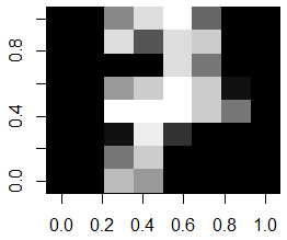
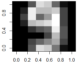
Each row in traindata and testdata is an image. Viewing an image can be done as follows; here we are viewing the 31st training image, which happens to be an image of the digit 7:
row.id <- 31
m <- matrix(as.numeric(traindata[row.id, 1:64]), nrow=8, ncol=8)
image(m[,8:1], col=grey(seq(0, 1, length=16)))
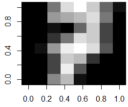
In order to visually see how much variation there is per digit, we could find all same digits in the training set, say all digits 7. Then we compute the average image for digit 7 and display this:
# select all training images for digit 7
train.7 <- traindata[traindata[,65]==7, 1:64]

# compute the average image from all the training images of digit 7
average.7 <- matrix(as.numeric(colMeans(train.7)), nrow=8, ncol=8)

image(average.7[,8:1], col=grey(seq(0, 1, length=16)))
If we want to visually compare and contrast two digits to each other, we can compute their average image, and subtract the two average images to find the differences. Here we illustrate this for digits 7 and 9:
train.9 <- traindata[traindata[,65]==9, 1:64]
average.9 <- matrix(as.numeric(colMeans(train.9)), nrow=8, ncol=8)

# show the difference image of digits 7 compared to 9
image(abs(average.7 - average.9)[,8:1])
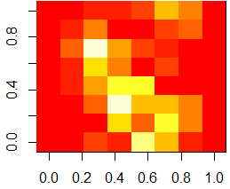
As one can see from the above difference image, the most distinguishable differences between digits 7 and 9 lie within the lower triangular part of the image.
\(k\)-NN classifier
One of the simplest classifiers is the \(k\) Nearest Neighbour (k-NN) classifier. In R, an implementation of the k-NN classifier is available in package class.
Usage of this classifier is very simple:
require('class')
# try with k = 1
pred <- knn(traindata[,1:64], testdata[,1:64], traindata[,65], k=1)
# compute the accuracy of this classifier
mean(pred == testdata[,65])
# generate the confusion matrix
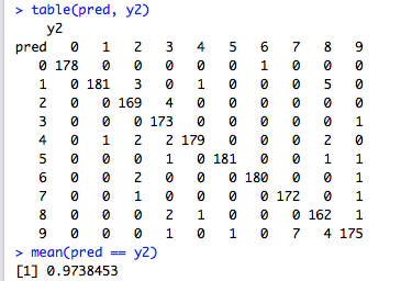
table(pred, testdata[,65])
With \(k\)=1
For evaluating the performance of the classifier (\(k\) set to 1), we rely on 2-fold cross validation, using the train-test split created by the dataset’s authors. The average performance of this classifier is of 97.9%.
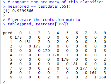
The Confusion Matrix allows us to look for pairwise confusion amongst the category labels (digits in this case). For example, we can see that this classifier confuses three instances of real 9’s as 8’s. There’s also an image of a 4 and another of a 1 that are also confused as an 8 (i.e., the classifier thinks they are an 8, while in actual fact they are a 4 and a 1 respectively). From this confusion matrix, one can also note that digits 0 are classified correctly with no errors (no false positives and/or false negatives).
Finding best value of \(k\)
What’s the optimal value of \(k\) for this dataset? Let’s try out with various values of \(k\) and then we compare classifier accuracy.
res = matrix(nrow=100,1)
for (k in 1:100)
{
	pred <- knn(traindata[,1:64], testdata[,1:64], traindata[,65], k)
	res[k] <- mean(pred == testdata[,65])
}

# plot the accuracy
plot(res, type='l', xlab='k', ylab='classifier accuracy', main='Accuracy vs. k for k-NN Classifier')
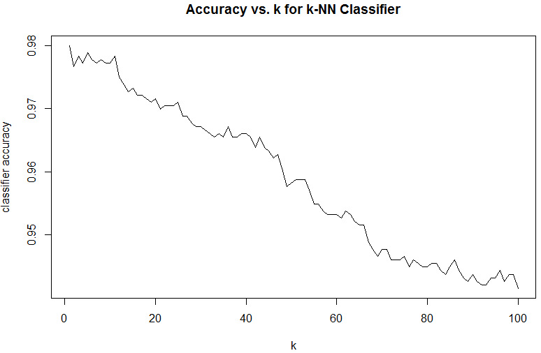
From the above graph, one can see that the best performing classifier is 1-NN, the simplest nearest neighbour classifier.
SVM classifier
Our next experiment in classification will make use of the Support Vector Machine (SVM).
We will use the e1071 package in R. This package provides an interface to the well-known libsvm library.
trn <- data.matrix(traindata)
tst <- data.matrix(testdata)

require(e1071)
When we try running SVM on the given optdigits training data, the following error will occur:
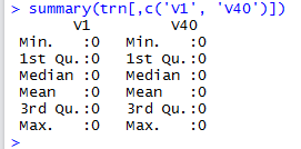
This error occurs because columns 1 and 40 happen to be always 0 for all the given training images, as can be confirmed by running summary() on the 2 columns:
We thus need to remove these 2 columns from the data used to train the SVM model. Note also how we cast the label column (the target column) to type factor. This is required in order
to indicate that the SVM is going to be used for classification purposes (Y values are categorical) and not for regression.
ndx <- c(2:39, 41:64) # we eliminate the all-zeros columns
# train the SVM model
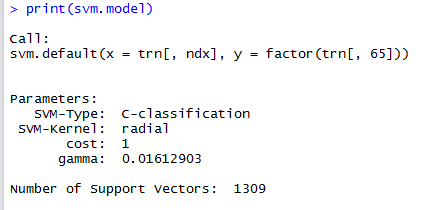
svm.model <- svm(trn[,ndx], factor(trn[,65]))
Leaving the svm() call with its default parameters results in the following SVM model:
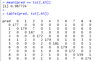
Now we run the SVM model on the test data in order to check the model’s accuracy.
pred <- predict(svm.model, tst[,ndx])
This is quite straightforward, and we compute the accuracy as well as the confusion matrix:
Tuning the SVM
We can see that the performance of the SVM classifier is worse than that of the Nearest Neighbour classifier (\(0.968\) against \(0.980\)). A question we can ask is the following: can we tune the SVM’s parameters
in order to improve the classification accuracy? cost and gamma are the parameters of the non-linear SVM with a Gaussian radial basis function kernel.
A standard SVM seeks to find a margin that separates the different classes of objects. However, this can lead to poorly-fit models in the presence of errors and for classes that are not that easily separable.
To account for this, the idea of a soft margin is used, in order to allow some of the data to be “ignored” or placed on the wrong side of the margin.
Parameter cost controls this: a small cost value makes the cost of misclassification low (soft margin) and more points are ignored or allowed to be on the wrong side of the margin, while a large value makes the cost of misclassification high (hard margin) and the SVM is stricter when classifying the points which can potentially lead to over-fitting.
Parameter gamma is a free parameter of the radial basis function.
To find the optimal values for parameters cost and gamma, we use the tune() method. This employs a grid search technique to locate the optimal parameter values and uses 10-fold cross validation in the process.
This method can be quite time-consuming. In machine learning this process of ‘tuning’ a classifier via finding the best parameter values is called hyperparameter optimisation.
tune.result <- tune(svm, train.x = rbind(trn[,1:64], tst[,1:64]), train.y = factor(c(trn[,65], tst[,65])), ranges = list(gamma = c(0.006, 0.008, 0.010, 0.012, 0.014), cost = c(3.25,3.5,3.75,4,4.25,4.5,4.75))
print(tune.result)
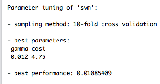
plot(tune.result)
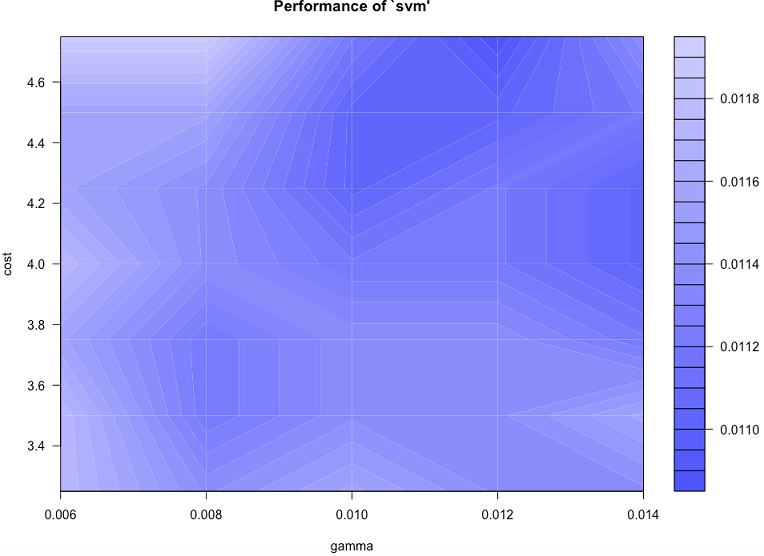
We can continue re-tuning and zooming further into the hyperparameter space until we reach a good level of accuracy.
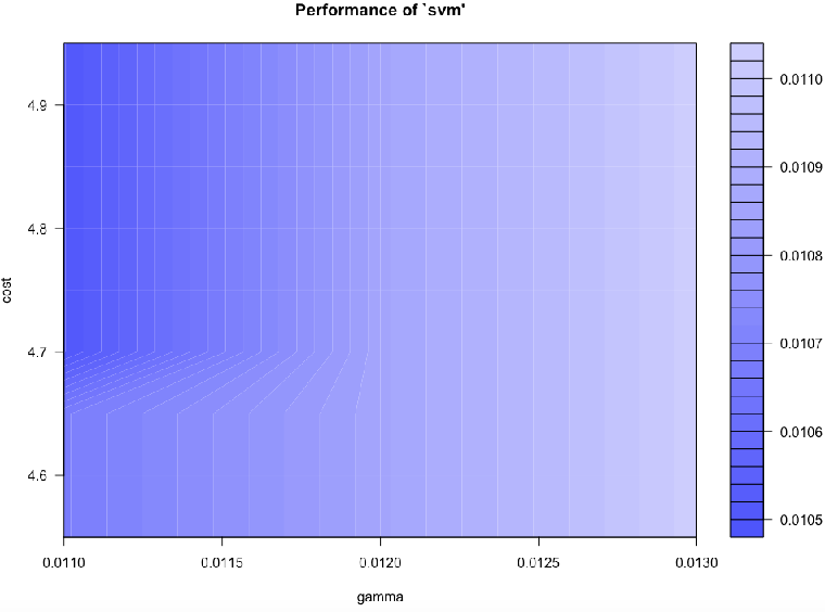
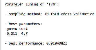
svm.model <- svm(trn[,ndx], factor(trn[,65]), gamma=0.011, cost=4.7)
pred <- predict(model, tst[,ndx])

mean(pred == tst[,ndx])
table(pred, tst[,ndx])
The final accuracy of the SVM classifier is still worse than that of the nearest neighbour (\(0.974\) against \(0.980\)), but hyperparameter tuning has gone a long way in improving the results of the SVM classifier (\(0.974\) against \(0.968\)).
Self-Organising Map (SOM)
The next classifier we tried is the Self-Organising Map (SOM). This is a special type of a neural network that makes use of unsupervised learning in order to generate a low-dimensional (2D in our case) representation of the data. This low-dimensional representation is called a map. SOMs are also known as Kohonen networks.
Here we make use of two R packages called Rsomoclu and Kohonen. Package Rsomoclu provides
an R interface to the library Somoclu.
require(Rsomoclu)
require(kohonen)

trn <- data.matrix(traindata)
tst <- data.matrix(testdata)
There are several SOM parameters that need to be configured before we can generate the map. For many of them, the default values can be used. The first two parameters nSomX and nSomY define the size of the 2-dimensional map.
nSomX <- 100
nSomY <- 100
nEpoch <- 10
radius0 <- 0
radiusN <- 0
radiusCooling <- "linear"
scale0 <- 0
scaleN <- 0.01
scaleCooling <- "linear"
kernelType <- 0
mapType <- "planar"
gridType <- "rectangular"
compactSupport <- FALSE
codebook <- NULL
neighborhood <- "gaussian"
Training and generatin the SOM can then be done via the following code:
som.res <- Rsomoclu.train(trn[,1:64], nEpoch, nSomX, nSomY,  radius0, radiusN,  radiusCooling, scale0, scaleN,  scaleCooling,  kernelType, mapType, gridType, compactSupport, neighborhood, codebook)

som.map = Rsomoclu.kohonen(trn[,1:64], som.res)
An important thing to note is that we do not pass the target labels as input to the SOM - remember that SOM uses an unsupervised learning method.
SOM Visualisations
SOMs in R come with a number of plotting options to help in visualising the map as well as checking its quality.
Let’s first take a look to see how the ten clusters of hadwritten digits have been organised by the SOM. We are going to use the known labels of the training images and see where they fall in the 2D map. We will use colour coding to help in the visualisation of the clustering. The following code does this:
require(RColorBrewer)

col.ind <- trn[,65] + 1
cols <- brewer.pal(10, "Paired")
cols[1] <- 'lightskyblue3'
cols[9] <- 'thistle4'

plot(som.map, type="mapping", labels=trn[,65], col=cols[col.ind], font=2, cex=1.5)
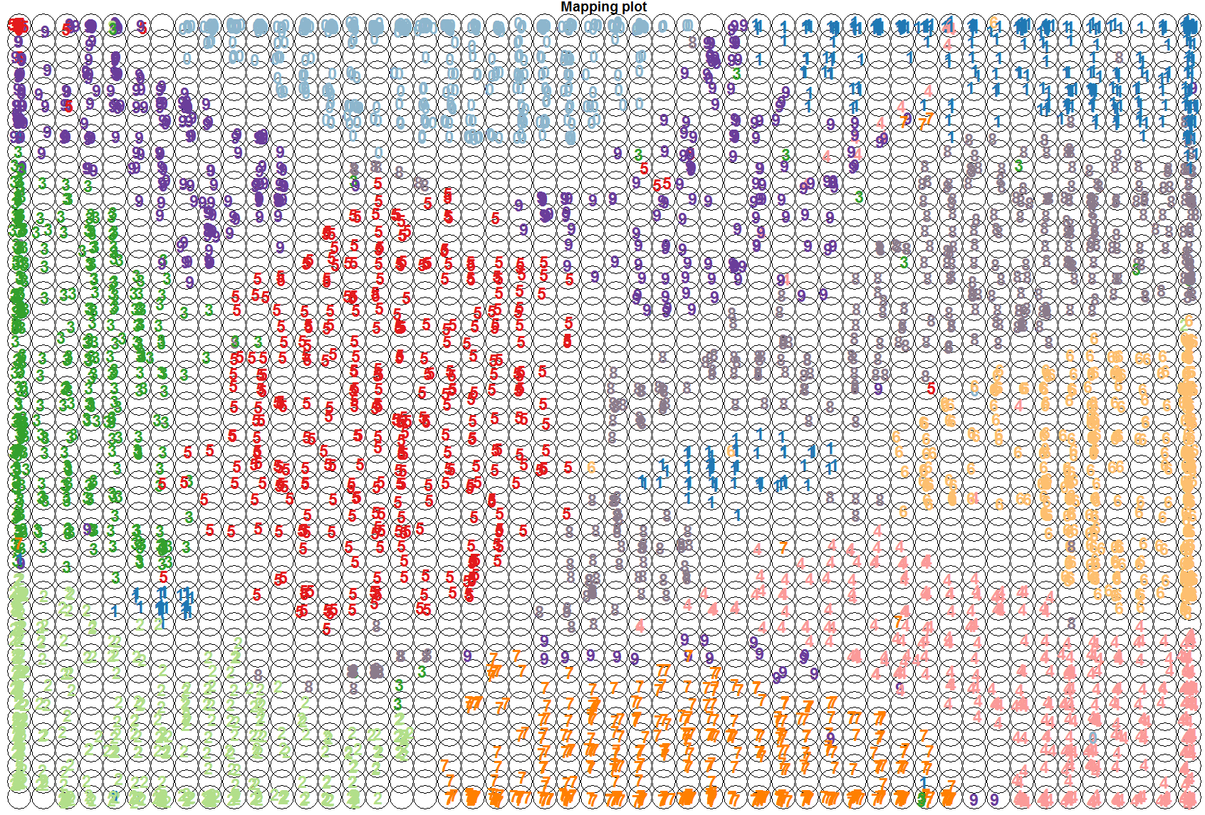
Note how the SOM has managed to cluster the digits quite well, keeping in mind that we have not supplied the target labels of the images; we only supplied the 64 pixel counts for the 8x8 blocks.
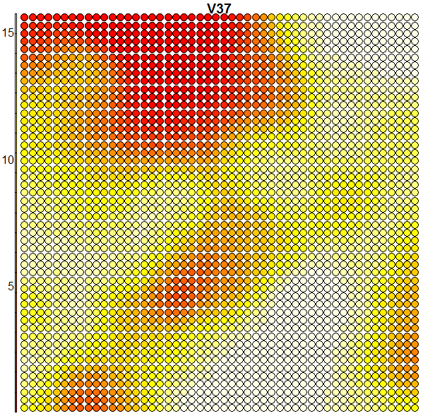
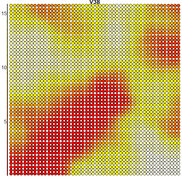
Heatmaps are perhaps the most important visualisation element of SOMs. A SOM heatmap allows the visualisation of the distribution of a single variable (single feature) across the map. For example, imagine we want to check how much the 36th column (i.e. the pixel counts of the 36th block) helps to discriminate the various clusters we have:
plot(som.map, type = "property", property = som.map$codes[,36], main = colnames(trn)[36])
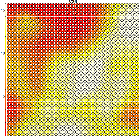
When we compare the above heatmap with the clusters mapping plot, we can see that the pixel totals of the 36th column are low for roughly digits 0’s and 9’s, while high for digits 1’s, 7’s and 8’s. The contours in the heatmap do not map well with the digit clusters. But remember that this is just the heatmap of one column – when an SOM clusters the input it takes into consideration all of the input data (all the 64 dimensions in this case). And perhaps column 36 is not such a good discriminator on its own. Some more examples of heatmaps are shown below:
The SOM library in R also provides other visualisations that can help with checking the quality of the generated map. For example, a neighbour distance plot (also known as the U matrix), and a plot of how many of the input images are mapped to each node on the map. Please check the package manual for more details.
Performance
Using the SOM for classification purposes can be done as shown here:
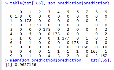
som.prediction <- predict(som.map, newdata=tst[,1:64], trainY=factor(trn[,65]))

mean(som.prediction$prediction == tst[,65])
With a 100x100 SOM, we obtained an accuracy of \(0.94769\).
In order to find the best size of the map, we evaluated a range of map sizes using the following code. We have restricted ourselves to square-sized SOMs here:
score = matrix(nrow=100,1)
for (s in seq(4,100,2))
{
   nSomX <- s
   nSomY <- s
   print(s)

   res <- Rsomoclu.train(trn[,1:64], nEpoch, nSomX, nSomY,  radius0, radiusN,  radiusCooling, scale0, scaleN,  scaleCooling,  kernelType, mapType, gridType, compactSupport, neighborhood, codebook)

   som.map = Rsomoclu.kohonen(trn[,1:64], res)
   som.prediction <- predict(som.map, newdata=tst[,1:64], trainY=factor(trn[,65]))
   score[s] <- mean(som.prediction$prediction == tst[,65])
   print(score[s])
}
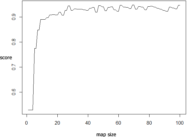
The best accuracy of \(0.9482471\) is obtained for a SOM size of \(70\)x\(70\).
We then performed another test to see what is the best value for the epoch parameter. Trying out with a range of epoch values varying from 10 to 150, we found out that the best result is obtained at
epoch = \(50\). With this epoch value, classification accuracy reaches \(0.96272\).
And the resulting map is given below (click on the image for a larger version). Please note that the map changes on each and every run, since SOMs are non-deterministic, but the same accuracy is obtained for different runs with the same configuration parameters.

From a training image to its SOM location
Before we leave the topic on SOMs, you might ask: is it possible to determine where on the map a particular image falls? Yes, we can do that.
The generated som has an element called unit.classif (accessible via som.map$unit.classif) that gives the number of the SOM node to which the training image belongs to.
For example, checking the first training image (first row in traindata),
(unit.num <- som.map$unit.classif[1])
we find out that this image is mapped to SOM node 2120. We reach the 2120’th node, by starting from bottom-left corner of the map and moving in a row-order fashion. The following code changes from node number to x,y coordinates (origin is at the bottom-left corner):
coord <- c(unit.num %% nSomX, unit.num %/% nSomX)
That’s all on SOMs for now.
Artificial Neural Networks
The next classifier that I tried is the venerable artificial neural network (ANN for short).
We will be using the R package neuralnet.
For this classifier, I opted for having 10 output nodes, one for each of the 10 handwritten digits. As a result, the dataset needs to be modified slightly to cater for this. The following code adds 10 extra columns at the end, one column per digit, and named ‘zero’, ‘one’, ‘two’, up to column ‘nine’. Each column takes a value of 0 or 1 depending on whether that row (that image) is of that particular digit or not.
traindata <- read.table("optdigits.tra", sep=",")
testdata <- read.table("optdigits.tes", sep=",")

for (k in 0:9)
{
    traindata <- cbind(traindata, (traindata$V65 == as.character(k)) + 0)
    testdata <- cbind(testdata, (testdata$V65 == as.character(k)) + 0)
}

names(traindata)[66:75] <- c('zero','one','two','three','four','five','six','seven','eight','nine')
names(testdata)[66:75] <- c('zero','one','two','three','four','five','six','seven','eight','nine')
For the network topology, we are using a 3-layer feed-forward network, consisting of an input layer of 64 nodes (the pixel totals for all the 8x8 blocks), a hidden layer of 70 nodes, and an output layer of 10 nodes (one per handwritten digit).
Model formulae
When it comes to specifying the statistical model of a machine learning algorithm, R provides a convenient syntax for specifying the model in terms of model formulae. Here our model for the neural network consists of 64 input variables (input columns) and 10 output variables (output columns). The input variables are known as the predictor variables. And the output variables are known as the target variables, because these are the variables that the neural network is trying to learn to predict their values. Another way of seeing this is the following: the neural network is trying to learn/find a mapping from the input variables to the target variables – this is the essence of supervised learning.
R’s model formula is a syntactic way of representing the statistical model of a machine learning algorithm. It is written as follows; with the target variable(s) on the left hand side, and
the input variables on the left hand side, separated by the tilde operator ~.
target variable(s) ~ input variables(s)
Note that a model formula is a symbolic expression, defining the relationships between variables (a prediction relationship), rather than it being an arithmetic expression.
For our neural network, we could use the following model formula:
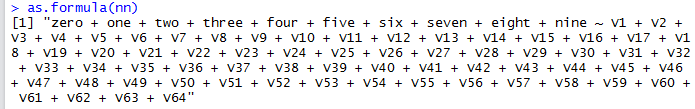
zero + one + two + three + four + five + six + seven + eight + nine ~ . - V65
We have the names of the ten target variables on the left-hand side. The + operator signifies the inclusion of an additional variable.
And as input on the right-hand side, we use the shortcut symbol ., which means include all variables not already mentioned in the formula (i.e. all variables
except for ‘zero’, ‘one’, up to ‘nine’).
But keep in mind that in our dataset we have an extra 65th column (named V65) that has the label of the handwritten digit. We have to remove this column from the input to the neural network,
and we do this by adding - V65 in the model formula, - signifying the exclusion of a variable.
This is the way we should specify the model for the neural network.
But unfortunately, the current implementation of neuralnet has a known bug in it.
When it encounters the symbol . in a model formula, it gives an error:
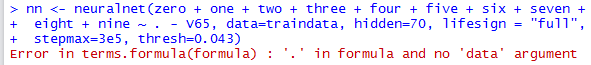
So we either have to specify it in full (listing all 64 input variables), or else specify it programmatically:
formula <- paste(paste(names(traindata)[66:75], collapse=' + '), '~', paste(names(traindata)[1:64], collapse=' + '))
Note that R provides a way to extract the model formula from a machine learning algorithm. We can use this as.formula() to verify
that the formula we created programmatically is correct (in this case nn is the neural network object):
Training the Neural Networks
Training the neural network is done as follows:
nn <- neuralnet(formula, data=traindata, hidden=70, lifesign = "full", stepmax=3e5, thresh=0.043)
Here we set the error difference threshold to \(0.043\). This means that the neural network will continue iterating and trying to find the best solution (i.e the ideal synaptic weights) till it reaches a point where the overall error of the model is not reducing by more than the given threshold value. In our case, if change in error at a given step of iteration is less than \(4.3\%\), the neural network will stop further optimization.
This neural network took quite some time to train, running for more than an hour. The good news is that you can train a neural network in stages (with saving to disk in-between stages). To do this, you can use the same method, with the addition that you pass to the method the weights from the previous training run:
# first training run
nn <- neuralnet(formula, data=traindata, ...)

# second training run
nn <- neuralnet(formula, data=traindata, ..., startweights = nn$weights)
Performance
The figure below shows a plot of the neural network that we have trained.
plot(nn)
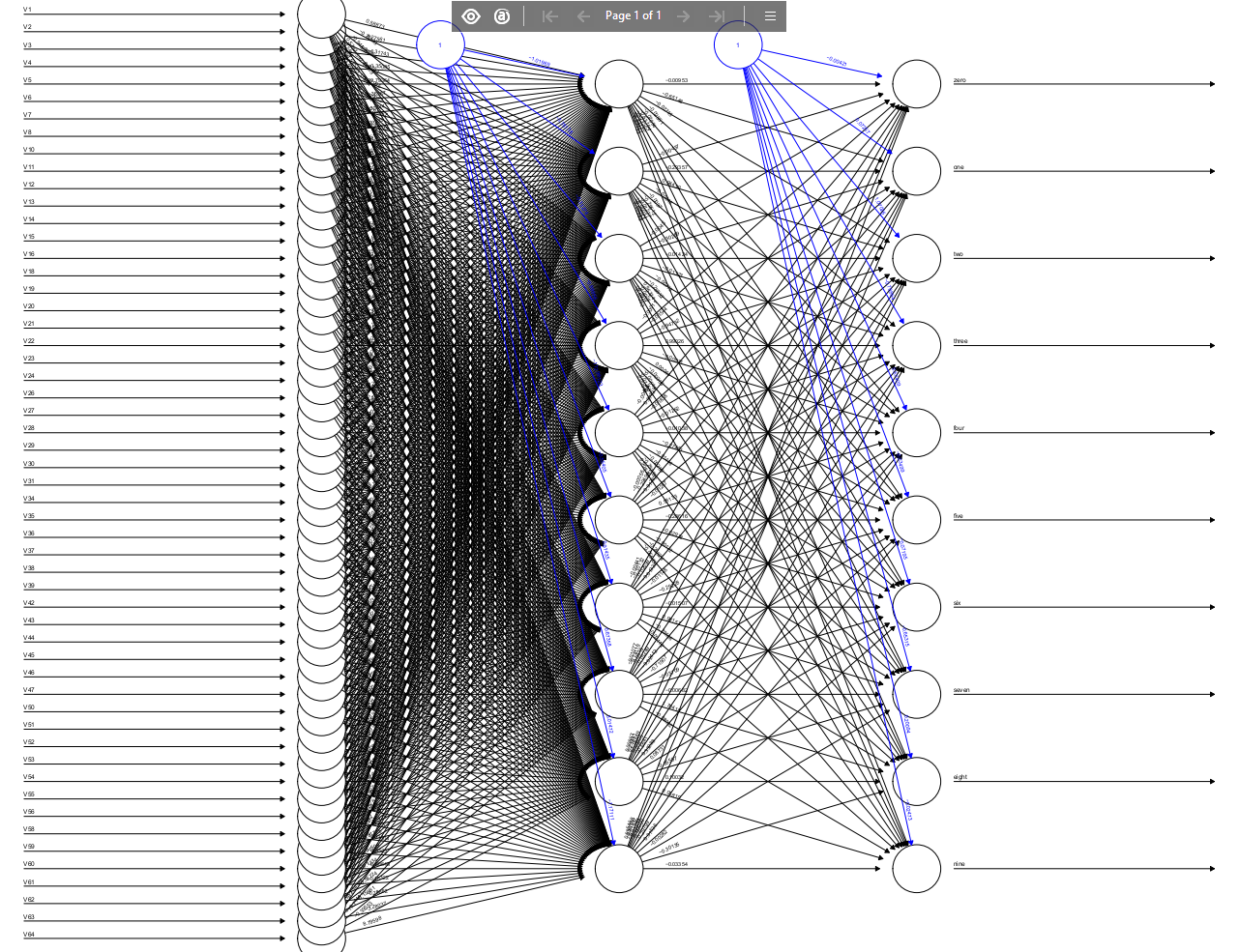
Since the neural network is quite large, the figure is very crowded and it’s hard to see the synaptic weights joining different nodes. It’s possible to customise the display of a neural network, for examply varying the width of the node connections to indicate weight strength – for more on this, please see this site.
Let’s now use the trained neural network nn to classify the test images. We’ll use the compute() method for this.
res <- compute(nn, testdata[,1:64])               # res$net.result will contain the output from all 10 output nodes of the neural network
pred <- apply(res$net.result, 1, which.max) -1    # for each test image, we find that output node which has the highest value and take this as the predicted output
res$net.result contains results from the 10 output nodes constituting the output layer of the neural network. We then apply which.max() on each row (each test image)
to find the output neuron with highest value. We take this as the predicted output of the neural network. We have to do -1 because indices in R start at 1, while our
handwritten digits start with zero.
We then compute the overall accuracy and the confusion matrix for the neural network classifier:
table(pred, testdata[,65])
mean(pred == testdata[,65])
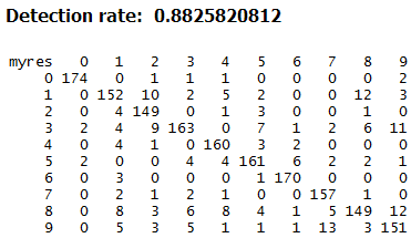
Neural networks are the worst performing amongst the classifiers we tried. Although to be fair, we have not tried doing any parameter tuning and/or topology optimisation. One reason for not doing this is the long time needed for training neural networks.
Random Forests
One final classifier that I am going to try in this post is Random Forests.
 Src: http://inspirehep.net/record/1335130/plots
Here we are going to use the R package randomForest.
Learning a random forest is quite straightforward:
require(randomForest)

rf <- randomForest(trn[,1:64], factor(trn[,65]), tst[,1:64], factor(tst[,65]), ntree=500, proximity=TRUE, importance=TRUE, keep.forest=TRUE, do.trace=TRUE)
We pass both the training and test folds of the dataset to randomForest(). It is important to note that we explicitly state that the target variables (the 65th columns) are
of type factor – without this, the random forest will default its execution mode to regression instead of classification. For the number of trees, we use the default value of
500 trees.
One of the main advantages of random forests is that they are very fast to train, while at the same time being powerful classifiers. A Random Forest is known as an ensemble method – it is a learning algorithm that constructs a set of classifiers (Decision Trees in this case) and then determines a final classification result by aggregating (summing up) the classification results of the individual classifiers. Methods of aggregation could include: taking a weighted vote, majority voting, etc. More information about the random forest implementation we are using can be found here.
Calling print on the random forest object rf provides some information about this ensemble method as well as confusion matrices. (Remember that we are passing the test dataset as input).
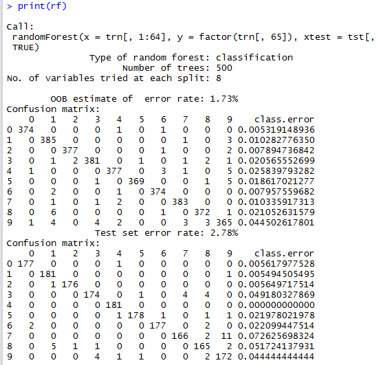
The first confusion matrix is for the training dataset, while second one is that of the test dataset and the one that is of interest to us.
Using the random forest rf for classification purposes is straightforward and the accuracy obtained is of \(0.97218\).
pred <- predict(rf, tst[,1:64])
mean(pred == tst[,65])

plot(rf)
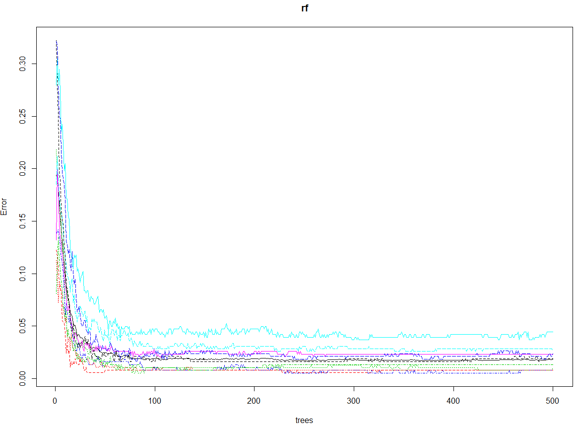
Note that we have not attempted doing any tuning of the random forest. Package randomForest has a method tuneRF() to assist in this process. This is something we can try in the future.
Importance of input variables
Analysing the workings of a Random Forest can yield several important insights on the problem in hand.
For example a call to importance(rf) will return a set of importance measures for each of the input variables. And when we call varImpPlot(rf) we
get a plot of the input variables ranked by their measure of importance:
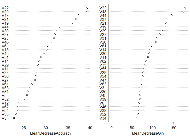
In the above plot we see the input variables ranked by two importance measures. The first measure is based on prediction accuracy averaged across all the trees making up the forest. The second measure is based on node impurity using the Gini coefficient – more information on these measures can be found here and here.
We can see that 5 most important input variables (the 5 variables that help most in classifying handwritten digits) are the pixel totals given in columns: 22, 43, 20, 21, and 19. This can be very useful information as it will allow us to determine what features (input variables) are most relevant to our problem. Note also that many of the input columns are left out from the above plot – these are variables that are not important for classification purposes; their presence provides little to none discriminating power to a classifier.
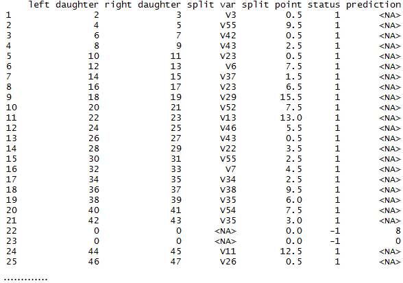
A Tree for You
The method getTree can be used to extract a given tree from the random forest rf. For example, in the code below, we are getting the 121st tree of the random forest.
# get a tree from the random forest
a.tree <- getTree(rf, 121, labelVar=TRUE)

print(a.tree)
Conclusion
To conclude this rather long blog entry, the table below summarises the accuracy results obtained and highlights some important characteristics of the classification algoithms that I have experimentd with.
| algorithm | accuracy | parameter tuning? | training speed | comments |
|---|---|---|---|---|
| k-NN | 97.997% | yes | fast | best result obtained for k=1 |
| SVM | 97.385% | yes | fast | used grid-search parameter tuning |
| Random Forest | 97.218% | no | fast | |
| SOM | 96.272% | limited | fast | unsupervised method |
| Neural Network | 88.258% | no | very slow |
That’s all folks!