Solving River-Crossing Puzzles with R
River-Crossing Puzzles are a popular class of puzzles in the field of AI. Many flavours of these puzzles exist. Here we use R to provide a somewhat generic framework to model and solve these type of puzzles.
River-Crossing puzzles
River-crossing puzzles are a type of puzzle where the objective is to move a set of pieces (objects, animals or people) across a river, from one bank of the river to the opposite bank, using a boat or a bridge. What makes these puzzles interesting are the set of rules and conditions that apply. Typically the boat is only able to carry a limited number of pieces at any one go. And normally there are rules and constraints that forbid having certain combination of pieces on the bank river and/or the boat.
Let’s look at an example.
The Farmer-Wolf-Goat-Cabbage riddle
Once upon a time, there was a Farmer who had a tiny boat. The boat was so tiny that it could only take the Farmer himself and one additional passenger. He wanted to move a Wolf, a Goat and a Cabbage across a river with his tiny boat.
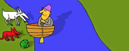
When the Farmer is around, everyone is safe, the Wolf will not eat the Goat, the Goat will not eat the Cabbage.
But he can’t leave the Wolf alone with the Goat because the Wolf will eat the Goat. He can’t leave the Goat alone with the Cabbage because the Goat will eat the Cabbage.
And of course he can only fit one more object with him on the boat (either the Wolf, the Goat or the Cabbage).
The question is: How can he safely transport the three of them to the other side of the river?
The Solution
Solving river-crossing riddles entails starting with all pieces on one side of the river (typically the left bank). This is the start state. Then one considers all possible valid moves that can be done given the start state. These possible moves create a set of new states. The process repeats itself with the new states until we eventually arrive at the goal state, i.e., having all the pieces safe and sound on the other side of the river.
In the table below I have listed a set of moves for the Farmer-Wolf-Goat-Cabbage riddle. We are using the symbols F, W, G, and C to stand for the Farmer, Wolf, Goat, and Cabbage respectively.
| move | left river bank | right river bank |
| Start state | F W G C | _ _ _ _ |
| Farmer takes the Goat to the right river bank | _ W _ C | F _ G _ |
| Farmer returns alone with the boat back | F W _ C | _ _ G _ |
| Farmer takes the Wolf to the right river bank | _ _ _ C | F W G _ |
| Farmer returns back with the Goat | F _ G C | _ W _ _ |
| Farmer takes the Cabbage across the river | _ _ G _ | F W _ C |
| Farmer returns back alone | F _ G _ | _ W _ C |
| Farmer takes the goat across. Exit state reached! | _ _ _ _ | F W G C |
As can be seen from the above table, this puzzle can be solved in 7 steps.
But is this the only solution there is?
To answer the above question we must build a graph of all possible valid moves. Thus we represent (model) the problem in terms of graph theory.
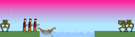
Then we can apply a graph search algorithm to find all possible paths from the start node to the goal node, the shortest path (smallest number of moves needed), etc. See the following video in order to apreciate the usefulness of this graph theoretic approach.
And talking of graphs, the R language has some great packages for solving graph related problems and performing graph analytics. One such package that I have used a lot is igraph. And I will be using this package in this blog to provide a solution to the river-crossing problems.
Generalising the solution
But before we start working on the solution, it is worthwhile remembering that River-Crossing puzzles come in many flavours and varieties.
This website lists many of these. For example, there is the Farmer-Fox-Chicken-Spider-Caterpillar-Lettuce puzzle where the farmer has to transfer 5 objects, but luckily for the farmer the boat is a bit larger (can carry 3 pieces). There are variants where a particular piece is repeated. For example, in the Farmer-2 Wolves-Dog-Goat-Bag of Grain puzzle we have 2 Wolves and they can eat both the Dog and the Goat.
Then there is the Japanese Family River-Crossing puzzle with its extremely complex rules. Also worth noting is the popular Missionaries-and-Cannibals problem, found in many AI text books.
Actually river-crossing puzzles are in themselves just a subset of the class of wider puzzles called the Transport Puzzles. But this is beyond the scope here - we will just concentrate solely on river-crossing puzzles.
R (igraph) solution
Keeping the above in mind, I opted to try and write as generic a solution as much as possible. After all, the ‘game’ mechanics are nearly the same for all puzzles. It’s only the rules and conditions that change. We will codify the rules separately from the rest of the code.
Defining the Conflict Graph
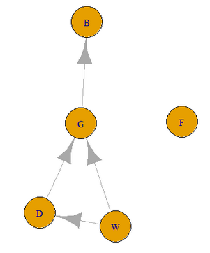
The rules and conditions that define the incompatibilites (conflicts) between the pieces can themselves be represented using a graph structure. For example in the Farmer-Wolf-Goat-Cabbage, the following graph encodes the rules:
- Wolf eats (conflicts with) Goat
- Goat eats Lettuce
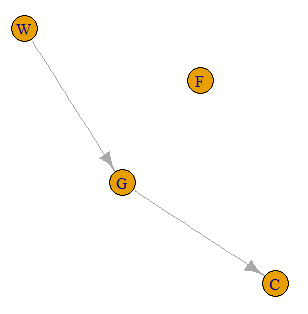
The following R code builds this conflict graph gr.
Note that in order to simplify the puzzle solving code, we add all the
pieces, even if they do not conflict with any other piece (F for the Farmer in this case.)
# the graph showing object incompatibilities
gr <- make_empty_graph(directed = TRUE)
gr <- add.vertices(gr, 4, name = c('F', 'W', 'G', 'C'))
gr <- add.edges(gr, c('W','G', 'G','C'))
plot(gr)
Also note that the conflict graph is a directed graph. Wolf eats Goat, but Goat does not eat Wolf - thus we define this as a directed edge (or directed arc in graph theory-speak).
Configuring the State Space graph
We now move on to the creation of the state space. This is the graph that will contain all valid states (states where no piece ends up as food and all rules of the game are observed).
We start with some configuration for this particular puzzle, and then create the empty graph gss that will store the state
space. Note that we created gss as a directed graph - actually using an undirected graph is also valid for a state space
graph.
boat.capacity <-2
farmer.symbol <- 'F'

gss <- make_empty_graph(directed=TRUE)
We have to define which of the pieces is the Farmer. Reason is that the code that generates the state space needs to know who will be rowing (handling) the boat. Only the Farmer can operate the boat.
We now create the graph node representing the start state as shown below and add it to the state space graph gss:
# create the initial state
state0 <- list(bank.l = c('F', 'W', 'G', 'C'), bank.r = c(), boat.pos = 1)
state0 <- make.state.name(state0)

# add the initial state as a node in the search space
gss <- add.vertices(gss, 1, name=state0$name)
V(gss)[1]$color <- 'red'
We adopt the following node structure for representing a state: each node consists of a list with 3 elements, bank.l, bank.r, and boat.pos.
bank.l is a vector containing the pieces that are on the left-hand side of the river, bank.r is contains those pieces
that are on the right-hand side, and boat.pos indicates where the boat is (1 for left-hand side, 2 for right-hand side).
In the case of the starting state, all pieces are on the left bank (bank.l) and the right bank is empty (bank.r is an
empty vector).
We must make a call to the function make.state.name for each state we create. This function constructs a string
that serves as a label to uniquely identify that state. For the start state, the string label is: CFGWb|. The pipe
symbol (|) represents the river and the symbols are placed on the left-hand side or the right-hand side of the pipe symbol
according to where they are located. The lower-case character b indicates where the boat is. To ensure consistent labelling of
nodes, the symbols for the pieces are sorted in alphabetical order.
Creating the State Space graph
Once we have the initial state defined, generating the full state space can be done via a simple call:
gss <- solve(gss, state0)
Function solve is defined in an R source file called solve_river_crossing_puzzles.R that can be downloaded
from here. I won’t go over the code contained in this source file - I think that
one can use it as it is without changes for the majority of river-crossing puzzles. Also, there are inline comments for
those brave enough to venture in.
After generating the state space graph, we make a call to igraph’s simplify() function. This removes any duplicate links
that might be created by the state space generation code. We also change the colour of the exit node and display the graph.
gss <- simplify(gss, remove.loops = FALSE, remove.multiple = TRUE)

V(gss)[startsWith(V(gss)$name, '|')]$color <- 'green'
plot(gss)
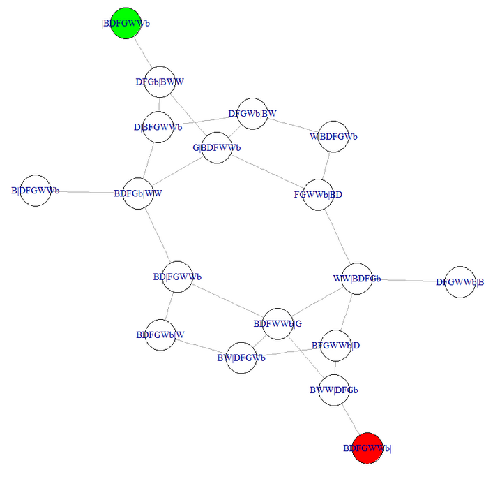
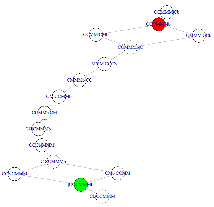
And here is the state space graph for the Farmer-Wolf-Goat-Cabbage puzzle:
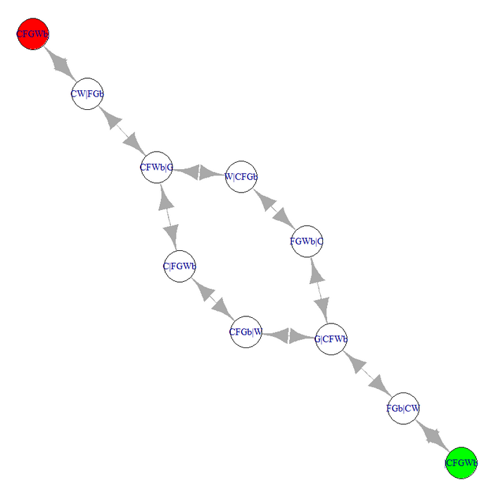
Note that a cursory glance at the above graph shows that there are 2 different solutions for this puzzle, both of length 7. But let’s use
igraph’s pathfinding functions in order to get these programmatically.
Finding solution paths
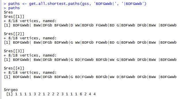
igraph has a function get.all.shortest.paths() that, given some node A and another node B, it finds all the shortest paths that connect node A to B.
In our case, we apply it to the start node and the goal node as shown below:
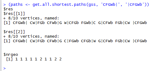
(paths <- get.all.shortest.paths(gss, 'CFGWb|', '|CFGWb'))
The output gives the required two paths:
If you find it a hassle to type in the labels of the start node and the goal node, you can use the following code instead. Although longer, this works for all puzzles, regardless of the symbols used and number of symbols.
(paths <- get.all.shortest.paths(gss, V(gss)[endsWith(V(gss)$name, '|')], V(gss)[startsWith(V(gss)$name, '|')]))
As one can notice, the hardest part in R is creating the state space. Finding the solutions leverages the power of the igraph package. Let’s apply our code to
some other more complex river-crossing puzzles.
The Farmer-Fox-Chicken-Spider-Caterpillar-Lettuce puzzle
This puzzle is similar to the previous one except that we now have 6 pieces and the boat can carry 3 pieces (the Farmer and any two other pieces).
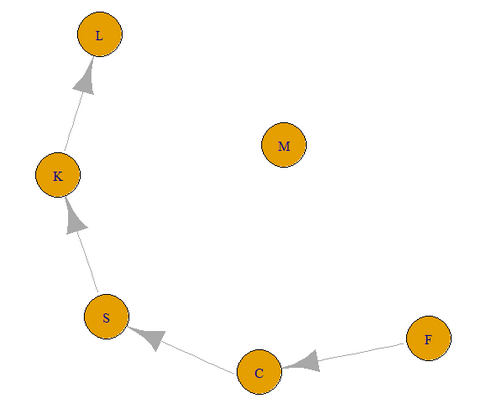
The conflict graph for this puzzle is given below. Note that we are using the following symbols: M = farmer, F = fox, C = chicken, S = spider, K = caterpillar, and L = lettuce.
# the graph showing object incompatibilities
gr <- make_empty_graph(directed = TRUE)
gr <- add.vertices(gr, 6, name = c('M', 'F', 'C', 'S', 'K', 'L'))
gr <- add.edges(gr, c('F','C', 'C','S', 'S', 'K', 'K', 'L'))
plot(gr)
We then create the state space graph as follows:
boat.capacity <- 3
farmer.symbol <- 'M'

# create the search space
gss <- make_empty_graph(directed=FALSE)

# create the initial state
state0 <- list(bank.l = c('M', 'F', 'C', 'S', 'K', 'L'), bank.r = c(), boat.pos = 1)
state0 <- make.state.name(state0)

# add the initial state as a node in the search space
gss <- add.vertices(gss, 1, name=state0$name)
V(gss)[1]$color <- 'red'

gss <- solve(gss, state0)

gss <- simplify(gss, remove.loops = FALSE, remove.multiple = TRUE)

V(gss)[startsWith(V(gss)$name, '|')]$color <- 'green'
plot(gss)
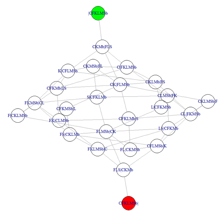
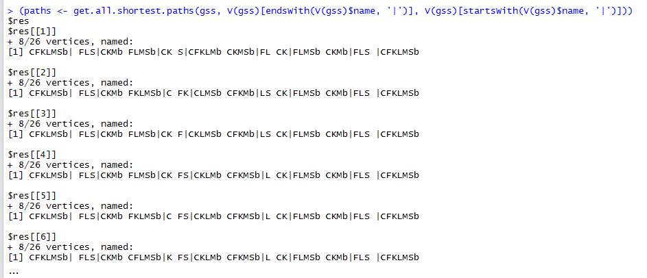
Note how complex (connected) the state space graph is! If we find all shortest paths, we get a total of 40 possible solutions, all of length 7. Only the first few are reproduced below:
(paths <- get.all.shortest.paths(gss, V(gss)[endsWith(V(gss)$name, '|')], V(gss)[startsWith(V(gss)$name, '|')]))
The 2 Wolves-Dog-Goat-and-Bag of Grain puzzle
This puzzle has a slightly more complex conflict graph as shown below. The symbols used are: F for Farmer, W for Wolf, D for Dog, G for Goat, and B for the Bag of Beans (Note that lower-case b represents the boat).
# the graph showing object incompatibilities
gr <- make_empty_graph(directed = TRUE)
gr <- add.vertices(gr, 5, name = c('F', 'W', 'D', 'G', 'B'))
gr <- add.edges(gr, c('W','D', 'W','G', 'D', 'G', 'G', 'B'))
plot(gr)
We then create the state space graph as follows:
boat.capacity <- 3
farmer.symbol <- 'F'

# create the search space
gss <- make_empty_graph(directed=FALSE)

# create the initial state
state0 <- list(bank.l = c('F', 'W', 'W', 'D', 'G', 'B'), bank.r = c(), boat.pos = 1)
state0 <- make.state.name(state0)

# add the initial state as a node in the search space
gss <- add.vertices(gss, 1, name=state0$name)
V(gss)[1]$color <- 'red'

gss <- solve(gss, state0)

gss <- simplify(gss, remove.loops = FALSE, remove.multiple = TRUE)

V(gss)[startsWith(V(gss)$name, '|')]$color <- 'green'
plot(gss)
This puzzle has a total of 4 possible solutions, again all of length 7.
The Missionaries and Cannibals puzzle
Now we come to a famous river-crossing puzzle that has different style of rules than the ones we have seen so far. Because of this we need to override some of the logic contained
in the source file solve_river_crossing_puzzles.R.
This puzzle is made up of 3 cannibals and 3 missionaries. A boat can carry at most 2 persons (anyone can operate the boat). If the number of cannibals on either side of the river outnumber the missionaries, then they will make a meal of the missionaries.
For this puzzle we need to consider counts of objects rather than conflicts between object types. Thus we will override the function is.bank.valid() that is called to check
whether the pieces on a bank’s river are according to the rules or not. We do the following:
is.bank.valid <- function(gr, state, side)
{
     b <- state[[side]]
     t <- table(b)
     num.c <- ifelse(is.na(t['C']), 0, t['C'])
     num.m <- ifelse(is.na(t['M']), 0, t['M'])
     return(num.m >= num.c | num.m == 0)
}
table() computes a histogram of the number of cannibals and missionaries on this side of the river. We have to handle NA’s for the cases where there are no missionaries or cannibals on this
particular river bank.
We also override the state transition checking in order to relax its strictness - anyone can operate the boat; the only rule is that the boat can not be empty.
# for this problem, the only rule is that the boat is not empty; thus override this method
is.transition.valid <- function(transition)
{
     return(min(is.na(transition)) == 0)
}
The code for creating the state space is similar to that of the previous puzzles:
boat.capacity <- 2

# the conflict graph - not used in this particular case; we will leave it empty
gr <- make_empty_graph(directed = TRUE)

# create the search space
gss <- make_empty_graph(directed = FALSE)

# create the initial state
state0 <- list(bank.l = c('M', 'M', 'M', 'C', 'C', 'C'), bank.r = vector(), boat.pos = 1)
state0 <- make.state.name(state0)

# add the initial state as a node in the search space
gss <- add.vertices(gss, 1, name=state0$name)
V(gss)[1]$color <- 'red'

gss <- solve(gss, state0)

gss <- simplify(gss, remove.loops = FALSE, remove.multiple = TRUE)

V(gss)[startsWith(V(gss)$name, '|')]$color <- 'green'
plot(gss)
The resulting state space graph is below:
Note that here we have 4 possible paths, all of length 11. Compare the above state space graph with the one shown on this page.
The Japanese Family River-Crossing puzzle
The final puzzle we will look at is the Japanese Family River-Crossing puzzle, which has some complex conflict rules. We have the Mom (M), Dad (D), 2 Daughters (D), 2 Sons (S), a Policeman (P), and a Thief (T). The rules of this puzzle are:
- The raft can carry no more than 2 people
- Only the Adults (Mom, Dad, Policeman) can operate the raft
- Dad can not be in the presence of the 2 Daughters without their Mom
- Mom can not be in the presence of the 2 Sons without their Dad
- The Thief can not be alone with any of the family without the Policeman
It’s difficult to represent the above conflicts with a single graph (at least I could not think of a way). Instead we will override the state generation logic as we did for the Missionaries and Cannibals problem. We end up with the following:
# for this problem, we need to consider complex incompatibilities between object types; thus override this method
is.bank.valid <- function(gr, state, side)
{
    b <- state[[side]]
    if (! is.element('M',b) & length(b) > 1 & is.element('F',b) & is.element('D',b))     { return (FALSE) }
    if (! is.element('F',b) & length(b) > 1 & is.element('M',b) & is.element('S',b))     { return (FALSE) }
    if (! is.element('P',b) & length(b) > 1 & is.element('T',b) & (is.element('F',b) | is.element('M',b) | is.element('S',b) | is.element('D',b)))     { return (FALSE) }

    return(TRUE)
}
We also need to override the state transition checks, since multiple persons can operate the boat:
is.transition.valid <- function(transition)
{
     return(is.element('M', transition) | is.element('F', transition) | is.element('P', transition))
}
The state space generation code is similar to that used in solving previous problems:
boat.capacity <- 2

# the graph showing object conflicts - not used in this particular case; leave empty
gr <- make_empty_graph(directed = TRUE)

# create the search space
gss <- make_empty_graph(directed = FALSE)

# create the initial state
state0 <- list(bank.l = c('F', 'M', 'P', 'T', 'D', 'D', 'S', 'S'), bank.r = vector(), boat.pos = 1)
state0 <- make.state.name(state0)

# add the initial state as a node in the search space
gss <- add.vertices(gss, 1, name=state0$name)
V(gss)[1]$color <- 'red'

gss <- solve(gss, state0)

gss <- simplify(gss, remove.loops = FALSE, remove.multiple = TRUE)

V(gss)[startsWith(V(gss)$name, '|')]$color <- 'green'
plot(gss, layout=layout.fruchterman.reingold(gss, niter=10000), vertex.label.cex=0.6)
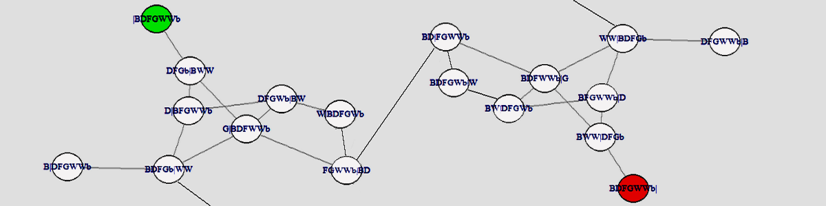
And the state space graph is shown below:
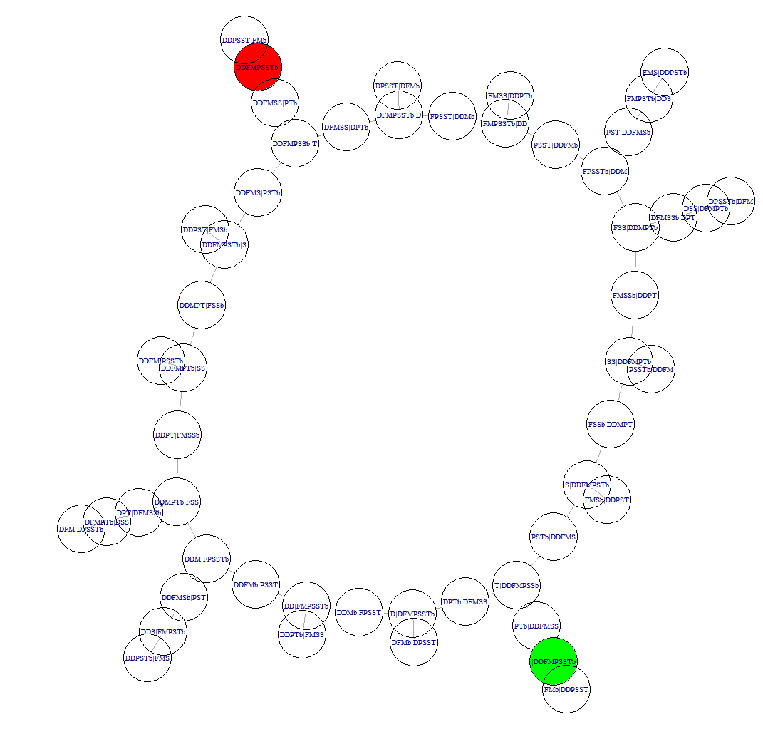
In this puzzle we have 2 possible shortest paths, both of lenth 17. Note also the number of side branches that terminate with a dead-end. A graph searching algorithm will have to use backtracking a number of times here.
Code repository
The code snippets used on this page can be found on github. There is also an R notebook that shows code usage, very similar to what has been done here.
Concluding Thoughts
I think that the given code provides a somewhat generalised solution to the river-crossing type of puzzles. It can be improved much further and also can benefit from improved packaging - something on my To-do list.
If you use the code, please acknowledgeb the source. Any improvements to the code are most welcome.
And for those that think that these puzzles are not really useful, there is a good book by Dr. Dave Moursund, titled Introduction to Using Games in Education: A Guide for Teachers and Parents. Also came across the following PhD on Games, Puzzles, and Computation, which shows the deep link between puzzles and mathematics and computing.
But perhaps the most important aspect is that they are fun to solve!