Predicting Customer Satisfaction

29 Apr 2016 • 14 min. read • Comments

The first Kaggle competition that I participated in dealt with predicting customer satisfaction for the clients of Santander bank. My submission based on xgboost was ranked in the top 24% of all submissions.

Kaggle ranks submissions based on unseen data – a public leaderboard dataset (test dataset with unseen targets) for use during development and a final private leaderboard dataset (completely unseen data) that is used for the final ranking of the competition.

In this blog I will cover some aspects of the work done, in particular, initial data exploration and balancing the dataset to aid machine learning predictions (happy customers far outweighed unhappy ones).

The input data

The input data consists of 369 anonymised features, excluding the ID column and the target column. So one problem with this competition was working in the blind about what each feature meant – thus little domain knowledge or intuition could be used.

Initial Data Exploration

The given training data is highly unbalanced. Exploring the frequency of the two target classes – 0 satisfied customers, 1 unsatisfied customers – one can see that less than \(4\%\) are unsatisfied customers. The dataset is highly imbalanced.

(t <- table(trn$TARGET) / nrow(trn))

require(plotrix)
l <- paste(c('Happy customers\n','Unhappy customers\n'), paste(round(t*100,2), '%', sep=''))
pie3D(t, labels=l, col=c('green','red'), main='Santander customer satisfaction dataset', theta=1, labelcex=0.8)

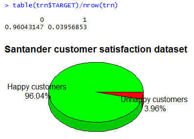
If we had to create a ‘classifier’ that simply outputs 0 (satisfied), we will get a \(96\%\) accuracy rate! Thus our baseline classification accuracy is \(96\%\) – we need to surpass this in order to have something useful.

To solve this we will balance the datasets to ensure that there is roughly the same proportion of satisfied to unsatisifed customers. But before doing that, let’s first clean the dataset.

Data Cleaning

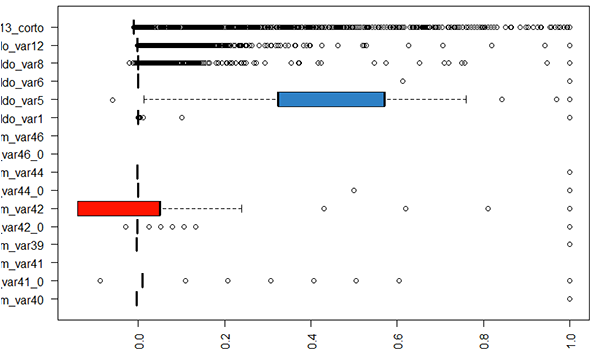
Using summary() on the dataset, we notice that there are several columns which have a single constant value – we can remove these. Boxplots are a very useful tool for checking this. There are also some columns which are identical to each other (duplicate columns) – these can also be removed.

# remove constant features
for (f in names(trn)) {
     if (length(unique(trn[[f]])) == 1) {
          cat(f, "is constant in train (", unique(trn[[f]]), "). We delete it.\n")
          trn[[f]] <- NULL
          tst[[f]] <- NULL
     }
}

# remove identical features
features_pair <- combn(names(trn), 2, simplify = F)
toRemove <- c()
for(pair in features_pair) {
    f1 <- pair[1]
     f2 <- pair[2]
   
     if (!(f1 %in% toRemove) & !(f2 %in% toRemove)) {
         if (all(trn[[f1]] == trn[[f2]])) {
             cat(f1, "and", f2, "are equal.\n")
             toRemove <- c(toRemove, f2)
         }
     }
}

feature.names <- setdiff(names(trn), toRemove)

trn <- trn[, feature.names]
tst <- tst[, feature.names[1:length(feature.names)-1]]

After performing the above, we end up with 306 features left, excluding the Target and ID columns.

Removing highly-correlated variables

A dataset with 306 variables is still too high. We will now look for strongly-correlated columns and leave only one in the training dataset. \(0.85\) is chosen as the threshold for high correlation.

# Removing highly correlated variables
cor_v <- abs(cor(trn))
diag(cor_v) <- 0
cor_v[upper.tri(cor_v)] <- 0
cor_f <- as.data.frame(which(cor_v > 0.85, arr.ind = TRUE))
trn <- trn[,-unique(cor_f$row)]
tst <- tst[,-unique(cor_f$row)]

image(cor_v)

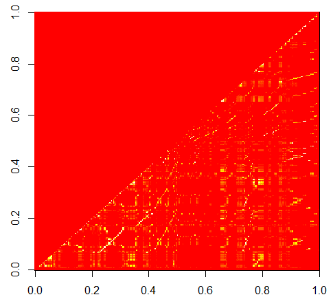
cor_v contains the pair-wise correlation of the columns and this is shown in the figure below. To remove highly-correlated columns, we take the lower triangle of cor_v and those that exceed the threshold are chosen for culling. We now end up with 143 features – much better than the original 369 features.

Balancing the Training dataset

As mentioned earlier, there is a massive mismatch between the number of satisfied customers (\(96\%\)) versus unsatisfied ones (\(4\%\)). We need to balance the 2 classes in order to avoid situations where a classifier can “learn” to always say “satisfied” when asked about a customer and is \(96\%\) of the time correct (the baseline accuracy).

We will use SMOTE for balancing the classes. SMOTE stands for Synthetic Minority Over-sampling Technique, and an implementation is available in the R package DMwR. The number of satisfied customers outnumber the unsatisfied ones by roughly a factor of 24 (24.27 to be exact). The code for performing balancing of the training dataset is given below:

require(DMwR)

# SMOTE requires the TARGET column to be a factor (not numeric):
trn$TARGET <- factor(trn$TARGET)

# Running SMOTE...
trn.bal <- SMOTE(TARGET ~., trn, perc.over=2427, perc.under=100)

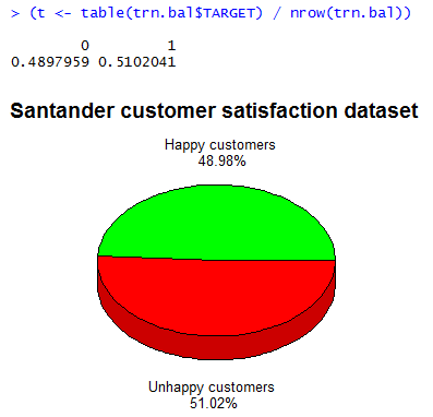
That’s it. Now both classes of customer types are approximately equal in number, as can be verified by re-generating the pie chart we did earlier:

Experiments in Predicting Customer Satisfaction

Decision Trees

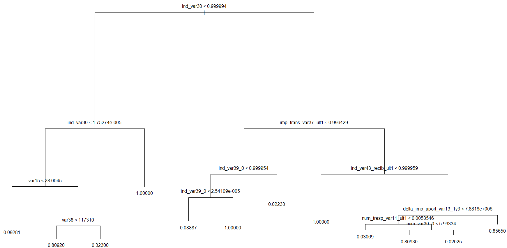
A decision tree was fitted to the balanced data set trn.bal as given below:

require('tree')

tr <- tree(TARGET ~., trn.bal)

plot(tr)
text(tr)

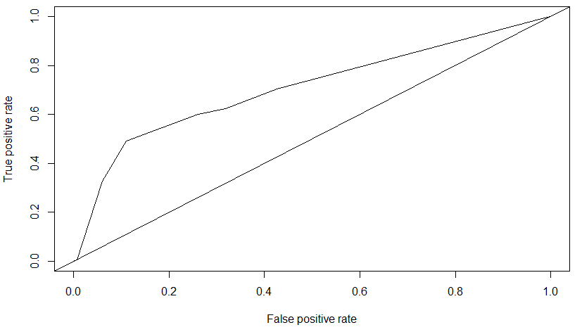
roc = performance(pred2, measure = "tpr", x.measure = "fpr")
plot(roc)
abline(a=0,b=1)

To evaluate the tree, the AUC metric (Area Under the Curve) applied to the ROC Curve (Receiver Operating Characteristic) was applied.

require(ROCR)

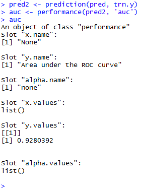
pred2 <- prediction(pred, tst$TARGET)
(auc <- performance(pred2, 'auc'))

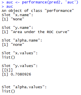
The AUC for this decision tree is \(0.70809\).

Support vector Machine (SVM)

Our next prediction experiment used an SVM.

We could not run the SVM on the full balanced dataset (147,392 rows), as it did not terminate after beibng left running for 24 hours. Thus we chose a subset of the training data (50,000 rows) randomly.

trn.bal.subset <- trn.bal[sample(nrow(trn.bal), 50000),]

trn.bal.subset$TARGET <- factor(trn.bal.subset$TARGET)

require(e1071)

# fit an SVM
model <- svm(TARGET ~., trn.bal.subset)

# do prediction
pred <- predict(model, tst[,1:ncol(tst)-1])

require(ROCR)
pred2 <- prediction(as.numeric(pred), tst$TARGET)
(auc <- performance(pred2, 'auc'))

roc = performance(pred2, measure = "tpr", x.measure = "fpr")
plot(roc)
abline(a=0,b=1)

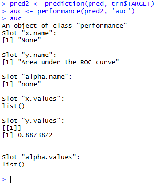
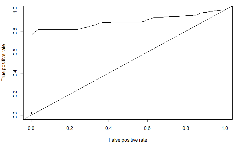
The AUC for the SVM trained on a subset of the balanced dataset is \(0.88739\). Though it is quite high, one can notice from the ROC curve that there are indications of over-fitting to the data. In fact, on the public leaderboard dataset of Kaggle, the SVM performed poorly - \(0.5758\). Compare this with the AUC value of \(0.7080\) of the Decision Tree on the public leaderboard.

XGBoost (eXtreme Gradient Boosted Trees)

XGBoost is a powerful gradient boosting technique used for decision tree ensembles.

One data preparation step is needed before we move on to Xgboost: We must ensure that the values of the variables of the test dataset do not exceed the minimum and maximum values of the variables in the training dataset. This is done as follows:

# extract the TARGET values
trn.y <- trn$TARGET
trn.bal.y <- trn.bal$TARGET

# remove the TARGET columns
trn$TARGET <- NULL
trn.bal$TARGET <- NULL

# limit vars in test based on min and max vals of train
print('Setting min-max lims on test data')
for(f in colnames(trn))
{
     lim <- min(trn.bal[,f])
     trn[trn[,f] < lim, f] <- lim
     tst[tst[,f] < lim, f] <- lim

     lim <- max(trn.bal[,f])
     trn[trn[,f] > lim, f] <- lim
     tst[tst[,f] > lim, f] <- lim 
}

# restore the TARGET values
trn$TARGET <- trn.y
trn.bal$TARGET <- trn.bal.y

We then build the Xgboost classifier using default parameters values for now.

library(xgboost)
library(Matrix)

set.seed(1234)


trn.bal <- sparse.model.matrix(TARGET ~ ., data = trn.bal)
dtrn.bal <- xgb.DMatrix(data=trn.bal, label=trn.bal.y)
watchlist <- list(train=dtrn.bal)

param <- list( objective              = "binary:logistic",
                     booster          = "gbtree",
                     eval_metric      = "auc",
                     eta              = 0.0202048,
                     max_depth        = 5,
                     subsample        = 0.6815,
                     colsample_bytree = 0.701
)

clf <- xgb.train(params       = param,
                    data      = dtrn.bal,
                    nrounds   = 3000,
                    verbose   = 1,
                    watchlist = watchlist,
                    maximize  = FALSE
)

# evaluate
pred <- predict(clf, tst)
require(ROCR)
pred2 <- prediction(pred, tst.y)
(auc <- performance(pred2, 'auc'))

roc = performance(pred2, measure = "tpr", x.measure = "fpr")
plot(roc)
abline(a=0,b=1)

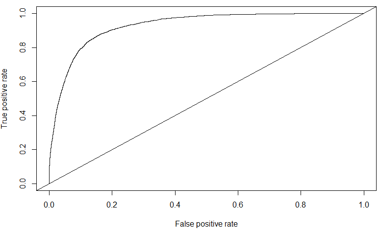
The AUC score obtained for Xgboost on the public leaderboard data is of \(0.828381\) – this is my highest for this competition, and ranked in the top \(24\%\) of all submissions. Further tuning of the Xgboost parameters might further improve this value.