Kaggle Shelter Animal Outcome Competition

In this blog I’ll go over some of my experiments on predicting the outcome of shelter animals. This work was done as my contributions to a competition on Kaggle.
One particular focus of this blog entry is on data exploration and feature engineering. This dataset had some interesting variables that needed some work before they could be used as predictor variables.
First of all, these are the machine learning algorithms that I tried out and the prediction accuracy obtained. Overall, my submission placed in the top 45% for this competition. This was my second time that I participated in a Kaggle competition.
| Machine Learning algorithm | Prediction Accuracy |
|---|---|
| SVM | \(73.05\%\) |
| Random Forest | \(67.09\%\) |
| Decision Trees | \(60.78\%\) |
| SOM | \(56.14\%\) |
Aim
The aim of this competition is to predict the outcome of animals (cats and dogs) that are kept in an animal shelter. The outcome could be one of:
- Returned to Owner
- Euthanised
- Adopted
- Transfered (to another centre)
- Died
Raw Data
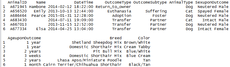
A sample of the training data is shown below:
trn <- read.csv('train.csv.gz')
head(trn)
Data Exploration
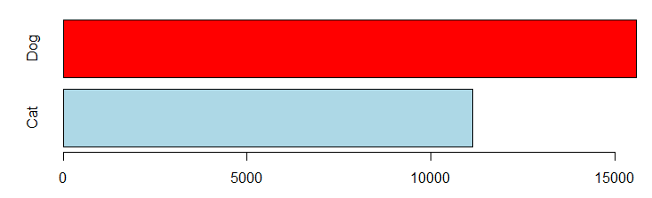
In the training dataset, there are more dogs than cats:
barplot(table(trn$AnimalType), horiz=TRUE, col=c("lightblue", "red"))
And the training data is not balanced by OutcomeType. Fortunately for the animals, not many of them are euthanised.
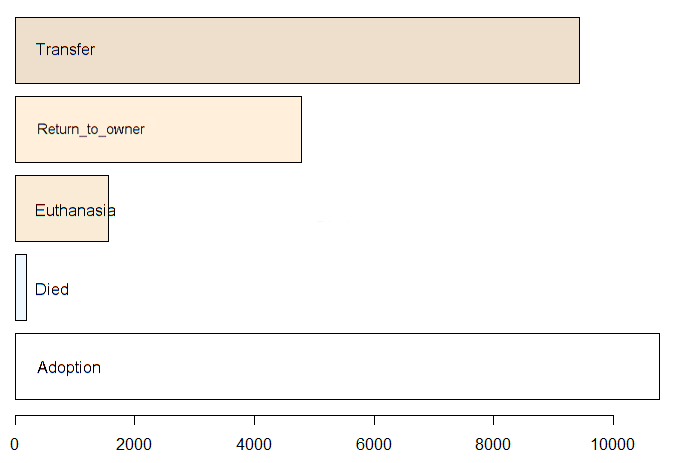
The following barplot shows the OutcomeType split by cats and dogs:
sweep(table(trn$OutcomeType, trn$AnimalType), 2,
	   colSums(table(trn$OutcomeType, trn$AnimalType)), "/")

barplot(table(trn$OutcomeType,trn$AnimalType),
	    col=c('red','yellow','orange','green','blue'), legend=TRUE)
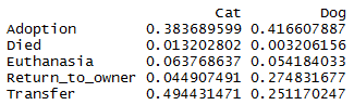
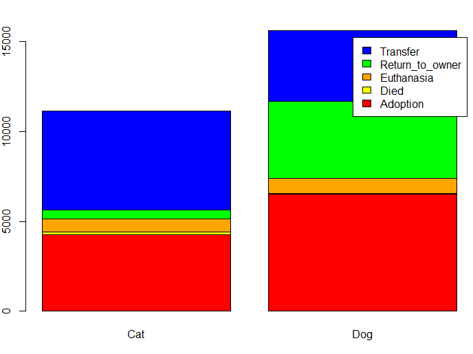
Note that many more dogs are returned to their owners than cats (\(27\%\) for dogs versus \(5\%\) for cats). Rate of euthanasia is approx the same. Rate of adoption is approx the same. Many more cats are transferred than dogs (\(49\%\) against \(25\%\)). Slightly more cats have died than dogs (\(1\%\) against \(<0.5\%\)).
Data Cleanup
We do some cleanup of the data. For example, the variable SexuponOutcome has both empty values and values with the
word Unknown – these mean the same thing.
trn$SexuponOutcome[trn$SexuponOutcome == ""] <- 'Unknown'
trn$SexuponOutcome <- factor(trn$SexuponOutcome)
Feature Engineering
Animal Age
The first column that needs modification is AgeUponOutcome. This is of string type and contains numbers and units expressed as words, e.g. “1 year”, “4 months”, “3 weeks”.
We need to change this to a numeric date range:
We split the age into 2 sub-strings and then convert the word representing the units to a singular word. After that we replace the units word with the corresponding duration in days. Finally, we compute the duration in days:
t1 <- sapply(as.character(trn$AgeuponOutcome), function(x)  strsplit(x, split=' ')[[1]][1])
t2 <- sapply(as.character(trn$AgeuponOutcome), function(x)  strsplit(x, split=' ')[[1]][2])

# replace 'weeks' with 'week'
t2 <- gsub('s','', t2)

# then replace "day" with 1, "week" with 7, etc
t2 <- ifelse(t2=='day',1,ifelse(t2=='week',7,ifelse(t2=='month',30,ifelse(t2=='year',365,-999))))

# now compute the duration in days
trn$AgeuponOutcome <- as.numeric(t1) * as.numeric(t2)
Now lets look at whether the OutcomeType shows any dependancy on the AgeuponOutcome variable:
barplot(table(trn$OutcomeType, trn$AgeuponOutcome),
	    col=c('red','yellow','orange','green','blue'), legend=TRUE)
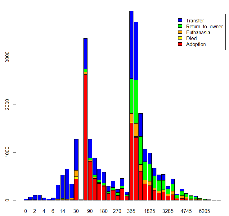
Many more outcomes happen at certain animal age.
Named Animals
How many animals have names?
barplot(table(trn$AnimalType, trn$Name != ""), horiz=TRUE, main="Animal has name?", col=c("blue","red"), legend=TRUE)
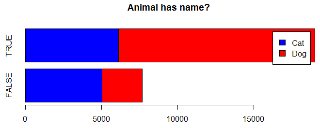
It appears that more dogs have names than cats.
Now, does the fact that an animal has a name affect its outcome?
barplot(table(trn$Name != '', trn$OutcomeType),
		main="Outcome versus an Animal having a name or not (T/F)",
		col=c("blue","red"), legend=TRUE, horiz=TRUE)
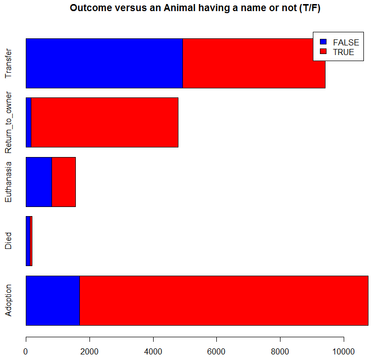
It appears that the fact that an animal has a name increases its chance of being returned to an owner and of being adopted. Thus we add a new predictor variable for this:
trn$hasName <- trn$Name != ''
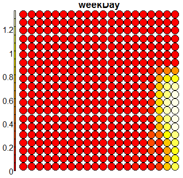
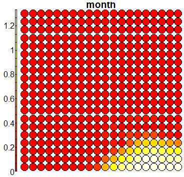
DateTime Features
There is a likelihood that the time of day, week day, and month affect the OutcomeType. Thus, we extract some new predictor
variables called timeOfDay, weekDay, and month, from the original DateTime feature.
# use a generic locale and time zone
Sys.setlocale("LC_ALL","English")

trn$DateTime  <- strptime(as.character(trn$DateTime),"%Y-%m-%d %H:%M:%S", tz="GMT")
trn$timeOfDay <- trn$DateTime$hour + trn$DateTime$min/60
trn$weekDay <- factor(weekdays(trn$DateTime))
trn$month <- factor(months(trn$DateTime))
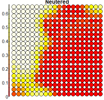
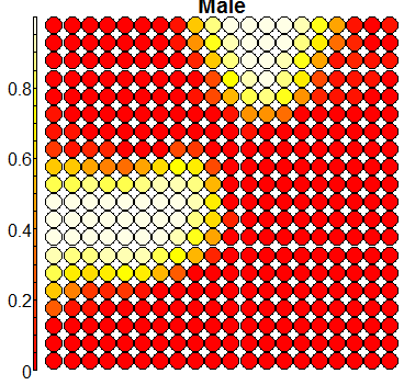
Sex and Neutered state
The original data has a variable called SexuponOutcome that takes the values: intact female, intact male, neutered male, spayed female, and unknown.
Since this feature variable encodes two signals together which could individually have some predictive power, I decided to split this into 2 separate predictor
variables.
trn$Neutered <- sapply(trn$SexuponOutcome, function(x) grepl('Neutered|Spayed',x))
trn$Male <- sapply(trn$SexuponOutcome, function(x) grepl('Male',x))
trn$SexuponOutcome <- NULL			# remove the original variables
Colour & Breed
The original Colour variable encodes 2 colours together, e.g., Brown/White, Orange Tabby\White, and Cream Tabby. Using the following code, we
split Colour into 2 variables Colour1 and Colour2:
trn$Color1 <- sapply(as.character(trn$Color), function(x) strsplit(x, split='/')[[1]][1])
trn$Color2 <- sapply(as.character(trn$Color), function(x) strsplit(x, split='/')[[1]][2])
trn$Color <- NULL
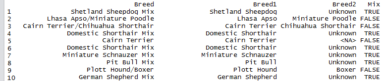
We do the same for Breed, with the addition that we create another variable called Mix to indicate those animals that are of a mixed breed.
trn$Breed1 <- sapply(as.character(trn$Breed), function(x) strsplit(x, split='/')[[1]][1])
trn$Breed2 <- sapply(as.character(trn$Breed), function(x) strsplit(x, split='/')[[1]][2])

# do we have a mixed breed as breed1 or breed2?
mix1 <- sapply(trn$Breed1, function(x) grepl('Mix', x))
mix2 <- sapply(trn$Breed2, function(x) grepl('Mix', x))
trn$Mix <- mix1 | mix2

trn$Breed2 <- ifelse(trn$Mix & is.na(trn$Breed2), 'Unknown', trn$Breed2)
trn$Breed <- NULL

trn$Breed1 <- gsub(' Mix', '', trn$Breed1)
trn$Breed2 <- gsub(' Mix', '', trn$Breed2)
Missing Data & Data Imputation
For the variables Breed1, Breed2, Colour1, and Colour2, we fill any missing values with the string Not Available.
For variable AgeuponOutcome, we use data imputation for filling in missing values by replacing them with the median of this variable:
trn$AgeuponOutcome[is.na(trn$AgeuponOutcome)] <- median(trn$AgeuponOutcome, na.rm=TRUE)
Self-Organising Map (SOM)
The first machine learning algorithm I tried is the Self-Organising Map. This is an unsupervised machine learning algorithm that can server
both as a dimensionality reduction visualisation tool as well as used for classification/prediction purposes. Rsomoclu is used.
require(Rsomoclu)
require(kohonen)
# convert the data frame to a matrix as required by the SOM
trn <- data.matrix(trn)
# scale the predictor variables so that all are of the same scale
trn[,1] <- scale(trn[,-1])
# configure the SOM parameters
nSomX <- 20
nSomY <- 20
nEpoch <- 10
radius0 <- 0
radiusN <- 0
radiusCooling <- "linear"
scale0 <- 0
scaleN <- 0.01
scaleCooling <- "linear"
kernelType <- 0
mapType <- "planar"
gridType <- "rectangular"
compactSupport <- FALSE
codebook <- NULL
neighborhood <- "gaussian"
# run the SOM
t1 <- Sys.time()
t1
res <- Rsomoclu.train(trn[,-1], nEpoch, nSomX, nSomY, radius0, radiusN,
radiusCooling, scale0, scaleN, scaleCooling, kernelType,
mapType, gridType, compactSupport, neighborhood, codebook)
sommap = Rsomoclu.kohonen(trn[,-1], res)
t2 <- Sys.time()
t2 - t1
# produce some visualisations
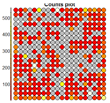
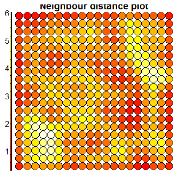
plot(sommap, type="dist.neighbours")
plot(sommap, type='counts')
# show the SOM clustering
require(RColorBrewer)
col.ind<-trn[,1]+1
cols <- brewer.pal(10,"Paired")
cols[1] <- 'lightskyblue3'
cols[9] <- 'thistle4'
plot(sommap, type="mapping", labels=trn[,1], col=cols[col.ind], font=2, cex=1.5)
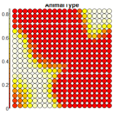
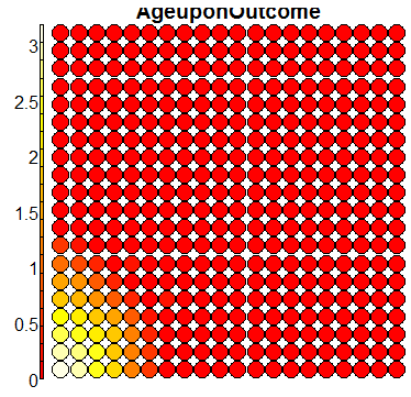
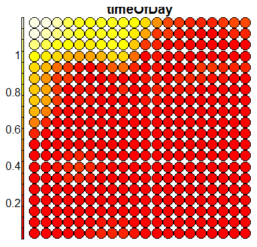
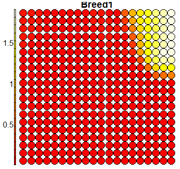
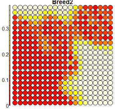
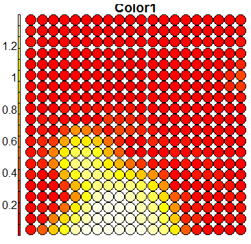
# plot the SOM heatmaps per predictor variable
for (k in 1:13)
{
plot(sommap, type = "property", property = sommap$codes[,k], main = colnames(trn)[k+1])
}
The first two plots are diagnostic plots which can be analysed to check the ‘quality’ of the generated SOM.
The next plot shows how the SOM has automatically clustered the training samples – the numbers and colours indicate different outcome types.
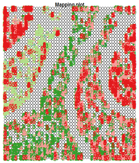
In the above figure, note how the training samples are not cleanly clustered into separate clusters. But there are some underlying patterns that indicate partial
clustering based on outcome type.
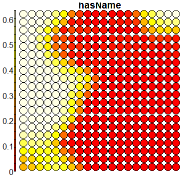
Compare this figure with the sequence of 13 heatmaps given below. Each heatmap represents a predictor variable. For example, the heatmap for variable hasName
has high-value regions (white) that coincide with the region of class 2 (return-to-owner) and parts of class 5 (adoption). Other patterns can also be seen in the other heatmaps.

Using SOM for prediction, gives a poor accuracy (\(56\%\)), mainly due to the fact that the clusters are not cleanly separable in the mapping plot.
som.prediction <- predict(sommap, newdata=trn1[,-1], trainY=factor(trn0[,1]))
table(trn1[,1], som.prediction$prediction)
mean(som.prediction$prediction == trn1[,1])
Random Forest
Our next machine learning algorithm is Random Forest. This is an ensemble-type classifier that makes use of bagging on 500 decision trees.
One limitation with the randomForest package of R is that it only allows up to 53 levels for categorical predictor variables. For Breed1 alone,
we have 220 distinct breed categories. Thus we need to reduce these category levels in order for random forests to work.
The following code orders the Breed categories by their frequency counts, selects ths top 52 ranked categories, and sets all the remaining breeds to Other.
br <- data.frame(table(all$Breed1))
br <- br[order(-br$Freq),]
nc <- br$Var1[1:52]               # we choose 52, because the 53rd will be the Others
all$Breed1 <- ifelse(all$Breed1 %in% nc, as.character(all$Breed1), "Other")
all$Breed1 <- as.factor(all$Breed1)

br <- data.frame(table(all$Breed2))
br <- br[order(-br$Freq),]
nc <- br$Var1[1:52]
all$Breed2 <- ifelse(all$Breed2 %in% nc, as.character(all$Breed2), "Other")
all$Breed2 <- as.factor(all$Breed2)

cl <- data.frame(table(all$Color1))
cl <- cl[order(-cl$Freq),]
nc <- cl$Var1[1:52]
all$Color1 <- ifelse(all$Color1 %in% nc, as.character(all$Color1), "Other")
all$Color1 <- as.factor(all$Color1)
Once we have taken care of this limitation, we can now train the random forest:
require(randomForest)

rf <- randomForest(x1, y1, x2, ntree=500, proximity=TRUE, importance=TRUE, keep.forest=TRUE, do.trace=TRUE)

# evaluate on the testing fold
pred <- predict(rf, x2)
table(pred, y2)
mean(pred == y2)
The average accuracy we obtain (using 5-fold cross-validation on the training set) is \(67.09\%\).
The random forest classifier can give us a ranking of the predictor variables by their importance – a variable with
high importance is able to offer more to the prediction of the outcome (higher discrimination). Running varImpPlot(rf) gives us the following figure:
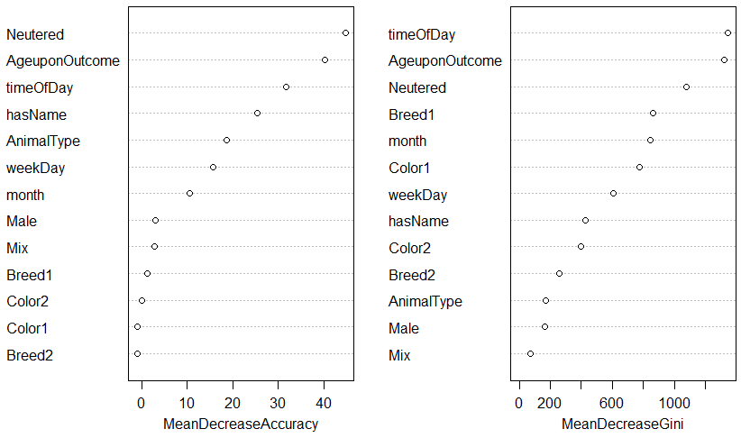
Note how Neutered, AgeuponOutcome, timeOfDay, and hasName contribute the most to the prediction, while the colour and breed variables contribute little.
Support Vector Machine (SVM)
We also tried an SVM classifier on this dataset, from the e1071 R package.
The SVM fails if the input data has NA's in it (missing values) – thus we must ensure that all missing values are set to Unknown or Not Available.
We used the caret package in order to use K-fold cross-validation on the training set. The createDataPartition() method ensures that all folds have
the same balance of the outcome types across all folds.
require(caret)

# define an 80%/20% train/test split on the training dataset
trainIndex <- createDataPartition(trn$OutcomeType, p=0.8, list=FALSE)
trn0 <- trn[ trainIndex,]
trn1 <- trn[-trainIndex,]
Training the SVM is done as shown below. The default radial basis function is used here, with the SVM set to C-classification mode, cost is 1, and gamma set to 0.002057613.
require(e1071)

t1 <- Sys.time()
t1
model <- svm(OutcomeType ~., trn0, probability=TRUE)
t2 <- Sys.time()
t2 - t1

# evaluation
x <- trn1[,2:ncol(trn1)]
pred <- predict(model, x, probability=TRUE)

table(pred, trn1$OutcomeType)
mean(pred == trn1$OutcomeType)
The prediction accuracy with the default SVM parameters is of \(63.735\%\).
SVM Tuning
The tune() method can be used for tuning the parameters of the SVM. This method performs a grid search with 10-fold cross-validation, which is computationally quite heavy.
t1 <- Sys.time()
t1
tuneResult <- tune(svm, train.x = OutcomeType ~ ., data = trn, ranges = list(gamma = seq(0,0.1,0.01), cost = seq(0.5,2,0.1)))
t2 <- Sys.time()
t2 - t1
A simpler and faster way to tune the parameters is given below:
gamma.range = seq(0, 0.1, 0.01)
cost.range = seq(0.5,2,0.1)

print(c("gamma.range", gamma.range))
print(c("cost.range", cost.range))

for (gamma in gamma.range) {
for (cost in cost.range) {
     print(c("gamma", gamma))
     print(c("cost", cost))

     t1 <- Sys.time()
     print(t1)
     model <- svm(OutcomeType ~., trn0, probability=TRUE, cost=cost, gamma=gamma)
     t2 <- Sys.time()
     print(t2)
     print(t2 - t1)

     x <- trn1[,2:ncol(trn1)]
     pred <- predict(model, x, probability=TRUE)

     print(table(pred, trn1$OutcomeType))
     print(mean(pred == trn1$OutcomeType))
}}
Note that the simpler method does not make use of K-fold cross-validation. Thus each time the above code is executed, the holdout set is different and so is the resulting SVM.
I opted for the simpler method, since the tune() method didn’t finish after being left to run for 24 hours!
The highest peak in accuracy in the searched parameter space occurred at the point where cost is \(1.6\) and gamma is \(0.09\). Evaluating on the test fold gave an accuracy of
\(73.05\%\). This is a marked improvement over the accuracy of \(63.735\%\) obtained with the default parameters, and highlights the importance of tuning the parameters of any machine learning algorithm.