Image Noise Modeling
A common assumption underlying many computer vision algorithms is that image noise is normally distributed. But is this a valid assumption?
Recently I was doing some investigations into error quantification and uncertainty estimation of computer vision algorithms. Many algorithms must rely on particular assumptions in order to be able to generalise well. Domingos (2012) does a good job at discussing this point and highlights that assumptions are an essential element of inductive learning and is what leads to the well-known bias effect.
A common assumption taken by many computer vision algorithms is that image noise is normally distributed, i.e., it follows a Gaussian probability distribution. And many times, these same algorithms are used without first ascertaining whether this assumption really holds or not. Personally I have done this a lot of times: blindly assuming that noise follows a Gaussian distribution.

But if such an assumption does not hold, then it can have repercussions on the accuracy of the results provided by algorithms. In the worst case an algorithm might “fail” outright because its workings are based on flawed foundations. In the best case, an additional error is introduced in the results giving rise to more uncertainty. As mentioned by Thacker (2003,2008), when it comes to determining the uncertainty of the results of an algorithm, one has to consider the input data and its assumptions.
Here are some of the results obtained from an investigation on the assumption of image noise normality.
Checking for Normality
To analyse image pixel noise, I used videos that have a static background, i.e., portions of the scene which are unchanging (no motion, no light variations) except for pixel noise.
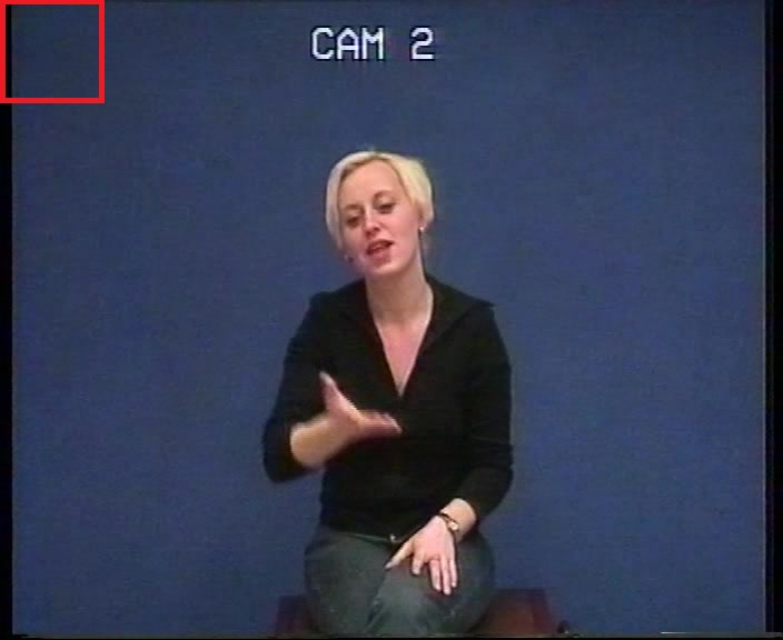
A frame of one of these videos is shown here, taken from the publicly-available ECHO Sign Language (NGT) Corpus , information on which can be found here. I will focus on a subset of pixels that occur within the highlighted red window. This window was chosen to be far away from the moving object in the video in order to eliminate as much as possible any interference between the foreground and the background. For pixels within the red window, their grayscale values over a temporal range of 1000 frames are read.
The R code for doing this is given below. The pixel values are stored in matrix pixel.data, where each column stands for a different pixel and contains its grayscale values over 1000 video frames.
Parameter colour.channel can be assigned one or more colour channels. If set to more than channel, e.g., 1:3, then the average value of the selected colour channels will be used.
require(jpeg)

video.path <- 'E:/VideoTestSequences/ECHO - Sign Language/NGT/Fables/NGT_AH_fab1/';
start.frame = 400;
end.frame =  1400;
colour.channel = 1:3;   # specify either a set of channels or a single channel
win.x = 1:50
win.y = 1:50

pixel.data <- NULL;

plot(1:2, main='image window used for image noise analysis');
for (n in start.frame:end.frame)
{
    video.frame.file <- paste(video.path, sprintf('%05d.jpg', n), sep='');
    video.frame <- readJPEG(video.frame.file);

    # take a window of the image
    img <- video.frame[win.y, win.x, colour.channel];

    if (length(dim(img)) == 3)
    {
        # we have multiple colour channels; change to grayscale
        for (k in 2:dim(img)[3])
        {
            img[,,1] = img[,,1] + img[,,k];
        }
        img[,,1] = img[,,1] / dim(img)[3];
        img <- img[,,1];
    }

    # display the window
    if (n %% 50 == 1)          # ... do this occasionally
    {
        rasterImage(img,1,1,2,2)
    }

    # change to a 1-dimensional array
    pixel.data <- rbind(pixel.data, as.vector(img));

    Sys.sleep(0.01)
}
We focus on the brightness values of a specific pixel for now. Since this pixel belongs to the static background it should have a constant value throughout the video sequence. That’s the ideal case. But in reality, due to noise effects, the pixel value will vary by some amount from frame to frame. This variation is shown in the figure below (pixel values have been normalised to the range 0 to 1):
![]()
The assumption is that this variation is Gaussian distributed with the mean of the distribution coinciding with the true value of the pixel. Many computer vision algorithms make this assumption and their workings rely on this assumption being true.
Now we will run a number of statistical tests, called normality tests, to check whether this assumption holds or not.
Shapiro-Wilk tests the null hypothesis (\(H_0\)) that the pixel values are drawn from a normally-distributed population. This is tested against the alternative hypothesis (\(H_1\)), that the pixel values are NOT normally distributed. To confirm the null hypothesis, the test statistic \(W\) returned by the Shapiro-Wilk test must be close to 1 and the probability value \(p\) must be above the chosen alpha value (0.05).
Another test is the Kolmogorov-Smirnov test, which compares the distribution of the given data against a normal distribution with mean and standard deviation derived from the data. For this test, the null hypothesis (\(H_0\)) is that both distributions are the same and having the same parameters, while the alternative hypothesis (\(H_1\)) is that the two distributions are different. In other words, the K-S test checks the following: if one had to approximate the data with a normal distribution, is the normal distribution a good enough approximation to explain the data? Do both have the same normal distribution with the computed mean and computed variance?
Finally, the skewness and kurtosis measures are computed for the pixel values. Skewness is a measure of symmetry, while Kurtosis is a measure of whether the pixel values are heavy-tailed or light-tailed relative to a normal distribution. Data with high kurtosis tend to have heavy tails, or outliers. Data with low kurtosis tend to have light tails, or lack of outliers. If the pixel data is normally distributed, then a skewness of 0 and a kurtosis of 3 is expected.
The R code below runs these normality tests on a given pixel.
run.shapiro <- function(d)
{
    res <- shapiro.test(d[1:min(1000,length(d))]);      # the Shapiro-Wilk test only works on a maximum of 5000 observations
    return(res)
}


plot_pixel_hist <- function(d, title='')
{
    # plot the histogram and fitted density
    brk <- ((floor(min(d)*255)-5) : (floor(max(d)*255)+5)) / 255;
    hist(d, probability=TRUE, breaks=brk, col='gray',
         main=paste('histogram of pixel values', title), xlab='normalised pixel values',
         sub='(blue: fitted density; red: Normal approximation)');
    lines(density(d), col='blue', lwd=2);

    # approximate the data with a gaussian
    dm <- mean(d);
    ds <- sqrt(var(d));
    dr <- seq(from=range(d)[1], to=range(d)[2], length=100);
    lines(x=dr, y=dnorm(x=dr, mean=dm, sd=ds), col='red', lwd=2);
}


analyse_pixel <- function(d)
{
    plot(d, pch=20, main='pixel values', xlab='frame #', ylab='normalised pixel value');
    cat(' \n\n');

    plot_pixel_hist(d);
    cat(' \n\n');

    qqnorm(d);
    qqline(d, col='red');
    cat(' \n\n');

    bp <- boxplot(d, main='Box-plot with Five Number Statistics',
                  sub='Open circles are outliers');

    # remove the outliers identified by the boxplot
    d2 <- d[d %in% setdiff(d, bp$out)];


    # Shapiro-Wilk test
    res <- run.shapiro(d);
    print(res)


    cat('skewness', skewness(d), '\n')
    cat('kurtosis', kurtosis(d), '\n\n')


    # Kolmogorov-Smirnov test
    res <- ks.test(d, "pnorm", mean(d), sqrt(var(d)))
    print(res);
}


pixel.no <- floor(length(img)/2);   # use the centre pixel of the window as an example

d <- pixel.data[,pixel.no];

analyse_pixel(d)
The figure below shows a fitted density to the pixel values (the blue curve) and the corresponding normal distribution (red curve) with mean and variance estimated from the pixel data.
![]()
The results of the normality tests are given in the table below:
| test | statistic | result | Expected for normality |
|---|---|---|---|
| Shapiro-Wilk test | \(W\) | \(0.98988\) | \(\approx 1.0\) |
| \(p\)-value | \(0.000002206\) | \(\gt 0.05\) | |
| Kolmogorov-Smirnov test | \(D\) | \(0.068162\) | |
| \(p\)-value | \(0.0001826\) | \(\gt 0.10\) | |
| Skewness | \(-0.1214216\) | \(\approx 0\) | |
| Kurtosis | \(3.720133\) | \(\approx 3.0\) |
From the above results, it appears that this particular pixel is NOT normally distributed. We have a rejection of the null hypothesis by both the Shapiro-Wilk test and the Kolmogorov-Smirnov test. In addition, we have some skewness and also kurtosis is not what one would expect for normally-distributed data.
The plot below shows a quantile-quantile (Q-Q) plot of the pixel data. For a normal distribution, the Q-Q plot should show the data points closely matching the diagonal red line with little deviation from it, especially at the far corners of the plot.
![]()
A look at the above Q-Q plot shows a “staircase” pattern caused by the quantisation of pixel brightness. This particular pixel only exhibits 52 unique discrete values over 1000 observations (video frames). The noise caused by quantizing the pixel values to a set of discrete values is known as quantization noise. We also observe some deviations in the tails of the distribution (the far corners of the plot).
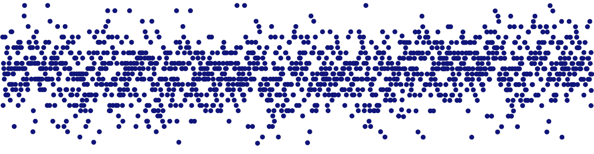
So far we have tested just one pixel for normality. The figures below summarise the results after performing the normality tests for all the pixels in the chosen window. Red indicates the pixels that fail the normality tests. As can be seen, the majority of pixels fail the test. Only \(5.4\%\) and \(9.8\%\) of the window’s pixels are normally distributed according to the Shapiro-Wilks and Kolmogorov-Smirnov tests respectively (these percentages are close to the alpha values chosen for the respective \(p\)-values).
![]()
Therefore we can conclude that while a normal distribution provides a good approximation to the fitted distribution of the pixel values (as can be seen from the histogram), the normality tests indicate otherwise. The Q-Q plot appears to show that the main culprit is quantisation.
Data Transformations
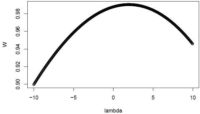
As a next step, a data transformation was applied to see if it can help to alleviate this problem and to see how the results of the normality tests are affected. We use Tukey’s Ladder of Powers transformations on the data to see if we can make it normally distributed.
pixel.no <- floor(length(img)/2); # use the centre pixel of the window as an example
d <- pixel.data[,pixel.no];

t <- transformTukey(d)
The results are still the same: the pixel data is reported as being non-normal by the Shapiro-Wilk test with a large confidence (\(p=0.0000043\)).
##
## lambda W Shapiro.p.value
## 470 1.725 0.9905 4.325e-06
##
## if (lambda > 0){TRANS = x ^ lambda}
## if (lambda == 0){TRANS = log(x)}
## if (lambda < 0){TRANS = -1 * x ^ lambda}
Dequantisation via Random Noise
Next we try to “undo” the quantisation effect by adding random noise to the pixel values. Here we are not interested in trying to recover the original non-discrete brightness values of the pixel, but only in “breaking” the quantisation effect. The random noise that we add to the original data is bounded by \(\pm 1\). The new histogram now looks like this:
![]()
We use the same R code as before to run the normality tests on the modified pixel values. The results of the normality tests are given below:
| test | statistic | original result | new result | Expected for normality |
|---|---|---|---|---|
| Shapiro-Wilk test | \(W\) | \(0.98988\) | \(0.99386\) | \(\approx 1.0\) |
| \(p\)-value | \(0.000002206\) | \(0.004013\) | \(\gt 0.05\) | |
| Kolmogorov-Smirnov test | \(D\) | \(0.068162\) | \(0.031138\) | |
| \(p\)-value | \(0.0001826\) | \(0.2863\) | \(\gt 0.10\) | |
| Skewness | \(-0.1214216\) | \(\approx 0\) | ||
| Kurtosis | \(3.720133\) | \(\approx 3.0\) |
For this particular pixel, the Shapiro-Wilk test is still reporting that the pixel values are not normally-distributed, but the Kolmogorov-Smirnov test is now saying that a Gaussian can be a good approximation to the given data. The Q-Q plot below is now showing a better situation with the “staircase” effect of quantisation no longer present. We can still see from the Q-Q plot that we have deviations from normality in the tails of the distribution (the corner areas in the Q-Q plot) and it is this that is causing the Shapiro-Wilk test to reject the null hypothesis. But as can be seen from the new histogram, a normal distribution can be a good enough fit for the pixel data – the Kolmogorov-Smirnov test confirms this by accepting the null hypothesis.
![]()
Applying this “dequantisation” technique to the rest of the pixels in the chosen window, we get the following results from the normality tests (yellow indicates pixels that pass the normality test).
![]()
As can be seen, the majority of pixels are now passing the Kolmogorov-Smirnov test, but not the Shapiro-Wilk test.
Conclusion
How one interprets the results of these investigations will depend on the computer vision algorithms in question. For example, in the case of background subtraction algorithms, personally I would base my interpretation on the Kolmogorov-Smirnov test. How well a normal distribution approximates the pixel values is the main factor for such background subtraction algorithms.
One has to keep in mind that this investigation has considered only a couple of videos that have their own limited characteristics. Similarly, sensors and cameras come in a variety of models each with its own particular characteristics. Illumination in a scene can vary a lot (like coherent and incoherent lighting). All these can exhibit various kinds of errors different from what is present in the videos considered here. We are ignoring correlations between pixels, compression artefacts, errors introduced by image processing on the camera device itself, etc. Generalising the above results must be done with great care.
References
P. Domingos, “A Few Useful Things to Know About Machine Learning,” Commun. ACM, vol. 55, no. 10, pp. 78–87, 2012.
N. A. Thacker et al., “Performance characterization in computer vision: A guide to best practices,” Computer Vision and Image Understanding, vol. 109, no. 3, pp. 305–334, 2008.
N. A. Thacker, “Using quantitative statistics for the construction of machine vision systems,” Proc. SPIE, vol. 4877, 2003.