t-SNE and Machine Learning
This blog continues on my previous entry on using t-SNE for exploratory data analysis. Now we will consider t-SNE for use within a machine learning system.
t-SNE and Machine Learning?
In my previous entry we saw that one disadvantage of t-SNE is that there is currently no incremental version of this algorithm. In other words, it is not possible to run t-SNE on a dataset, then gather a few more samples (rows), and “update” the t-SNE output with the new samples. One would need to re-run t-SNE from scratch on the full dataset (previous dataset + new samples). Thus t-SNE works only in batch mode.
But despite this disadvantage, it is still possible to use t-SNE (with care) within a machine learning solution. And the use of t-SNE can improve classification results, sometimes markedly.
Let’s outline a plan and then try it out on a real dataset to evaluate the accuracy improvement brought about by t-SNE.
- Given a training dataset and a test dataset, combine the 2 together into one full dataset
- Run t-SNE on the full dataset (excluding the target variable)
- Take the output of the t-SNE and add it as \(K\) new columns to the full dataset, \(K\) being the mapping dimensionality of t-SNE.
- Re-split the full dataset into training and test
- Split the training dataset into \(N\) folds
- Train your machine learning model on the \(N\) folds and doing \(N\)-fold cross-validation
- Evaluate the machine learning model on the test dataset
Steps 5 to 7 are your typical machine learning process. What we have added here is an earlier step whereby we run t-SNE on the full dataset (training + test), and then add the output of t-SNE as new features (new columns) to the dataset.
Due to the batch-mode operation of t-SNE, when we need to use the machine learning algorithm for predicting/classifying, unfortunately we need to repeat the full process (up to step 6) – the rows for which prediction is required now become the new ‘test’ dataset.
t-SNE with Random Forests
Let’s try it out on the optdigits dataset and using a Random Forest as a machine learning algorithm. In a previous blog entry, we found out that with Random Forests, we obtained an accuracy of \(97.218\%\).
require(randomForest)

rf <- randomForest(trn[,1:64], factor(trn[,65]), tst[,1:64], factor(tst[,65]), ntree=500, proximity=TRUE, importance=TRUE, keep.forest=TRUE, do.trace=TRUE)
Let’s reuse the same dataset and run t-SNE on it.
# load the datasets
traindata <- read.table("optdigits.tra", sep=",")
testdata <- read.table("optdigits.tes", sep=",")
trn <- data.matrix(traindata)
tst <- data.matrix(testdata)
# combine into one full dataset
all <- rbind(trn, tst)
# perform t-SNE
require(Rtsne)
tsne <- Rtsne(as.matrix(all[,1:64]), check_duplicates = FALSE, pca = FALSE, perplexity=30, theta=0.5, dims=2)
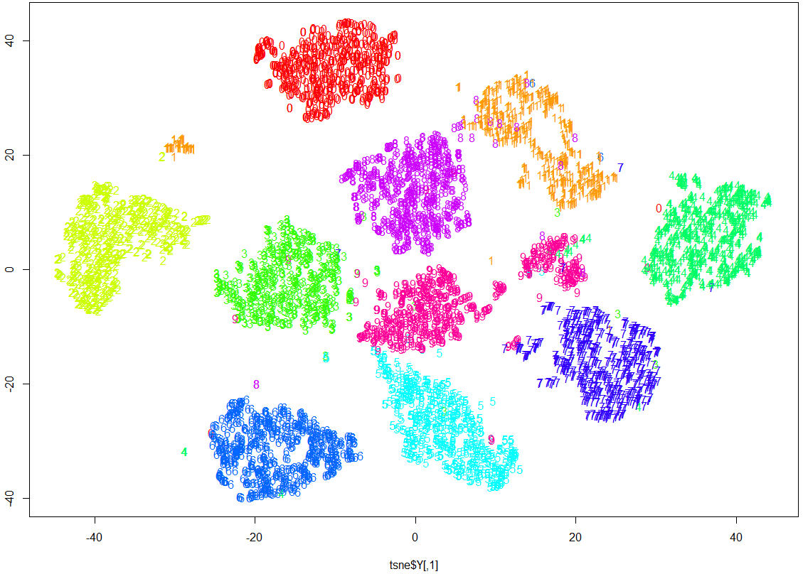
# display the results of t-SNE
cols <- rainbow(10)
plot(tsne$Y, t='n')
text(tsne$Y, labels=all[,65], col=cols[all[,65] +1])
Next we bind the map coordinates produced by t-SNE as new columns in the dataset. And we train a Random Forest on this enriched dataset:
# add the t-SNE map coordinates as new columns in the full dataset
all <- cbind(all[,1:64], tsne$Y, all[,65])

# now re-split into trn and tst
trn <- all[1:3823,]
tst <- all[3824:5620,]

# now the target label is in column 67 and columns 1:66 contain the input variables
x1 <- trn[,1:66]
y1 <- trn[,67]

x2 <- tst[,1:66]
y2 <- tst[,67]

# having unnamed input columns, gives an error while training a random forest
colnames(x1)[65:66] <- c("TSNEx", "TSNEy")
colnames(x2)[65:66] <- c("TSNEx", "TSNEy")

# train the random forest
require(randomForest)

rf <- randomForest(x1,factor(y1),x2,factor(y2), ntree=500, proximity=TRUE, importance=TRUE, keep.forest=TRUE, do.trace=TRUE)

pred <- predict(rf, x2)
table(pred, y2)
mean(pred == y2)
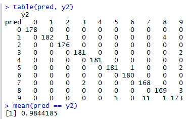
We can now see that the classification accuracy has increased from \(97.218\%\) to \(98.441\%\). In fact t-SNE + Random Forest is now my top-performing classification algorithm for the optdigits dataset.
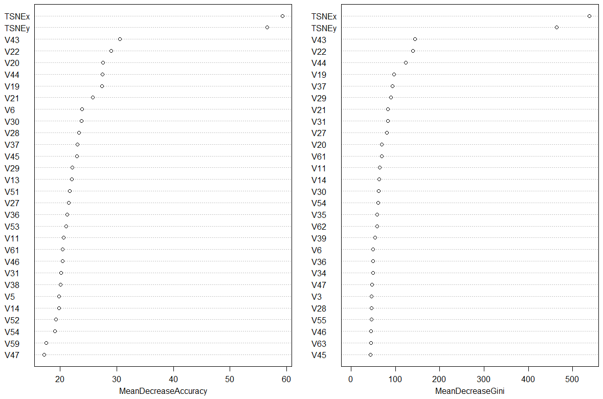
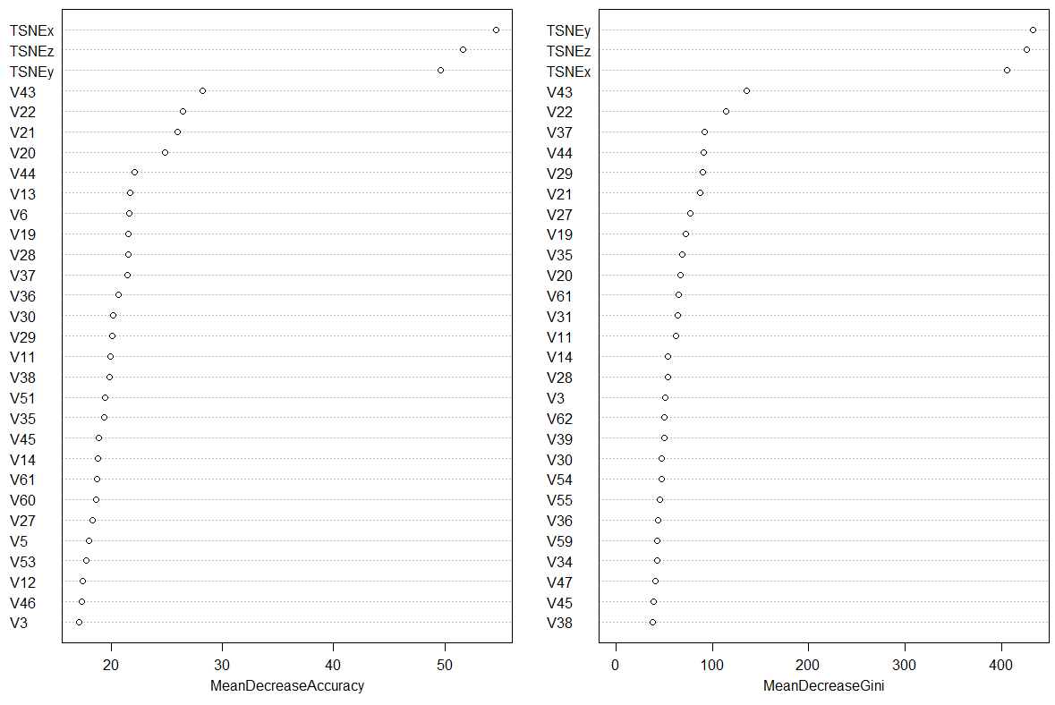
Are the t-SNE columns important?
Making a call to varImpPlot(rf) gives the following ranking of variables. Note how and by how much the random forest has found variables TSNEx and TSNEy to be of importance when classifying optdigits.
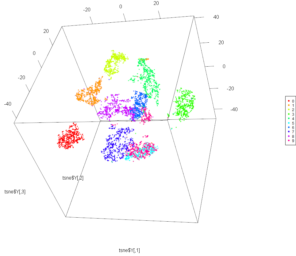
3D t-SNE and Random Forests
Let’s now repeat the experiment, but this time using t-SNE to reduce dimensionality to 3 instead of 2. The code is nearly identical, so we reproduce only parts which differ:
# dimensionality reduction to 3D (dims=3)
tsne <- Rtsne(as.matrix(all[,1:64]), check_duplicates = FALSE,
			  pca = FALSE, perplexity=30, theta=0.5, dims=3)

#display results of t-SNE
require(rgl)
plot3d(tsne$Y, col=cols[all[,68] +1])
legend3d("topright", legend = '0':'9', pch = 16, col = cols)
To aid visualisation of the 3D map, we can use R to generate a movie with the 3D plot spinning. The code below generates individual video frames as PNG files.
If ImageMagick is installed and parameter convert is set to TRUE, then a movie file is created instead. But so far, I could not get R to work correctly with
ImageMagick and thus had to rely on ffmpeg to combine the video frames together. Linking R with ImageMagick needs further investigation!
movie3d(spin3d(), duration=5, clean=FALSE, convert=FALSE, dir='c:/temp' )
# combine the dimensionality reduction coordinates of t-sne with the full dataset:
all <- cbind(all[,1:64], tsne$Y, all[,65])

# having unnamed input columns, gives an error while training a random forest
colnames(x1)[65:67] <- c("TSNEx", "TSNEy", "TSNEz")
colnames(x2)[65:67] <- c("TSNEx", "TSNEy", "TSNEz" )

rf <- randomForest(x1,factor(y1),x2,factor(y2), ntree=500, proximity=TRUE, importance=TRUE, keep.forest=TRUE, do.trace=TRUE)

pred <- predict(rf, x2)
table(pred, y2)
mean(pred == y2)
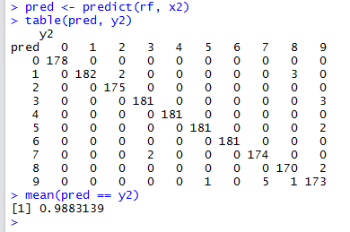
With 3D t-SNE output added as input to Random Forest, the classification accuracy has now increased to \(98.831\%\) – this is a massive improvement! And the importance of the t-SNE variables
is again evident from the varImpPlot figure:
3D t-SNE with Nearest Neighbour Classifier
Repeating the experiment with a Nearest Neighbour Classifier, we get an accuracy of \(98.664\%\) – again, a large improvement.
Below I am reproducing the accuracy table given towards the end of this blog post and adding the new results we obtained here. The great improvement that t-SNE adds to the machine learning solution is quite clear.
| algorithm | accuracy | parameter tuning? | training speed | comments |
|---|---|---|---|---|
| 3D t-SNE + Random Forest | 98.831% | no | no | |
| 3D t-SNE + 1-NN | 98.664% | no | no | |
| 2D t-SNE + Random Forest | 98.441% | no | no | |
| k-NN | 97.997% | yes | fast | best result obtained for k=1 |
| SVM | 97.385% | yes | fast | used grid-search parameter tuning |
| Random Forest | 97.218% | no | fast | |
| SOM | 96.272% | limited | fast | unsupervised method |
| Neural Network | 88.258% | no | very slow |
t-SNE on Shelter Animal Outcome dataset
In my previous blog entry, we saw that t-SNE didn’t produce a useful 2D or 3D visualisation for the Shelter Animal Outcome dataset.
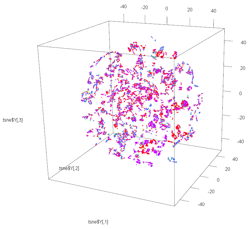
But let’s use 3D t-SNE and a Random Forest classifier just the same, and see if there is any change in accuracy. We will use 2-fold cross validation and use the Random Forest classifier as described in this post.
Below is the list of variables ranked by importance according to the random forest.
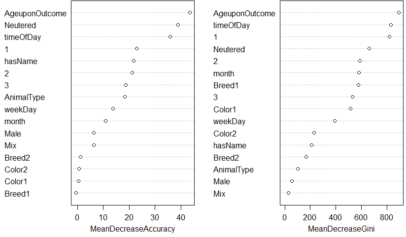
And the average accuracy after 2-fold cross validation is of \(67.26\%\) – this is a slight improvement over the \(67.09\%\) accuracy obtained by the random forest on its own.
Thus we can conclude that there is some discriminating power in the 3 variables TSNEx, TSNEy, and TSNEz and even the random forest thinks so. But is this small improvement in accuracy worth the batch mode processing limitation? It depends on the problem at hand.
Conclusion
To conclude, t-SNE can be integrated into a machine learning solution. If the t-SNE manages to cluster the data correctly, it can boost the accuracy of the machine learning solution quite drastically.